DCamProf - a digital camera profiling tool
Table of contents
- News
- What is DCamProf?
- Downloading DCamProf
- How DCamProf models cameras
- Basic workflow for making a DNG profile using a test target
- Basic workflow for making an ICC profile using a test target
- Basic workflow for making a profile from camera SSFs
- Choosing test target
- Test target reference files
- Shooting test targets
- White balance and camera profiles
- Tone curves and camera profiles
- Chromatic adaptation transforms in camera profiling
- Subjective looks in camera profiles
- Handling extreme colors
- File formats
- Command reference
- Report directory files
- Call for spectral databases and camera SSFs
- Acknowledgments
News
2018-11-30Version 1.0.6 is now released which is a maintenance release. It includes mainly bug fixes made within the commercial Lumariver Profile Designer project. No major new features backported at this time.
- More flexible and more robust CGATS parsing.
- More flexible tone curve parser.
- When ICC profile is made to apply white balance the forward matrix is now normalized so the sum of Y is kept at 1.0.
- The 1931 observer was by mistake mapped to Judd Vos 1978, now fixed.
- The si-render command now supports specifying band range for
indexed files using the new
-bparameter.
2017-05-22
During the past year I've worked with a graphical user interface to
DCamProf, which now is
available: Lumariver
Profile Designer. It's commercial software (not open-source and
costs money). DCamProf will still continue to be open-source, but the
main effort regarding support and features will be concentrated on
paying customers.
2017-01-17
Version 1.0.5 is now released which is just a hot-fix release. I've
become aware that the exclude patches and glare parameters for the
make-profile command became broken (=had no effect) in the 1.0.1
release, and I've fixed that in this release.
2016-10-10
Version 1.0.4
- Extended matrix optimization control to make-profile with the
new parameters
-vand-V. Now it's much easier than before to steer the optimizer in a custom direction if desired. - Now presenting hue errors with direction, just as lightness an
chroma.
- Hue is ordered magenta-red-yellow-green-cyan-blue, so if a red patch has a positive hue error it means that it's more yellow than it should be, and if it's negative hue error it's more magenta than it should be.
- Slight behavior change of
-lparameter to make-profile: now unnamed patches keep their default automatic relax ranges rather than get stuck at zero, plus it's now possible to provide a negative-to-positive range also for hue. - Now possible to address individual patches with
-land-wto make-profile, so you don't need to make patch classes if you don't need to group together patches. - Fixed some rounding errors in DE matching reports.
- Large updates to the make-profile command documentation to cover the new matrix optimization feature.
- Changed back the behavior of the
-Lto make-dcp so it skips both HueSatMap and LookTable. - Clearer error messages for conditions when gamut compression cannot be applied.
2016-09-29
Version 1.0.3 is now released. Fixed fatal bug in curve parsing
introduced in v1.0.2.
2016-09-27
Version 1.0.2 is now released.
- Added an extra (optional) HSV-based compression step to gamut
compression.
- Makes it feasible to achieve much stronger compression effects than previously, useful if you want to mimic the strong compressions found in many commercial bundled profiles.
- Two new presets added, "srgb-strong", "adobergb-strong", that uses the new pre-processing step that makes gamut compression much stronger. I expect "adobergb-strong" to be the most popular choice.
- If you have generated profiles with the previous "adobergb" preset, you may want to regenerate them with "adobergb-strong" preset to get more compression which makes it easier to work with high saturation subjects such as flowers.
- Allow gamut compression even with a linear curve.
- Now possible to provide "CurveMax" to a "Curve" look operator object if you want to specify the curve range in some other range than zero to one (usually zero to 255).
- Various code cleanups without functional change (maintenance).
- Added a new section in the documentation about how to relate to white balance presets.
2016-08-17
Version 1.0.1 is now released, and with it ready-to-run binary builds
for Windows (64 bit) and Mac OS X. It's so easy to build in Linux so
there you have to build from source. There's very little code changes
from the last release, only some minor bug fixes so if you already
have 1.0.0 installed there's no immediate need to update.
2016-05-20
Version 1.0.0 is now released. This is just a "rebranded" version of
the previous 0.10.5, no new functionality has been added. The
documentation on this page has got a much needed cleanup though.
DCamProf was originally pre-released in the end of April 2015, and an intensive period of adding new features and fixing bugs followed until November the same year. Since that six months have passed with more user testing, and I now think the software is stable enough to be promoted to version 1.0.0, which means that it's ready to be used by a broader audience.
Don't forget to check out the companion tutorial, Making a camera profile with DCamProf, which also has got a cleanup for this 1.0 release. The size of all this documentation may look a bit frightening — if you just want to make a good profile with the least possible effort, then go to the tutorial document and jump straight to the "easy way out" sections.
News archive
To keep down the size of this page the old news has been moved to a separate news archive page.
What is DCamProf?
DCamProf is a free and open-source command line tool for making camera profiles, and performing tasks related to camera profiles and profiling.
To make a camera profile you need either the camera spectral
sensitivity functions (SSFs) or a measured target. DCamProf has no
measurement functionality, but you can use the free and
open-source Argyll CMS to get a
.ti3 file with measurement data which DCamProf can read.
Here's a feature list:
- Generate camera profiles from test target measurements or camera spectral sensitivity functions (SSFs).
- Import (and export) measurement data from Argyll.
- Detailed control of matrix and LUT optimizers to hand-tune the trade-off between accuracy and smoothness.
- Test profile color matching performance, with free choice of illuminant.
- Save reports and data files for plotting (using gnuplot for example).
- Simulate reflective spectra all the way to the locus.
- Built-in spectral database with Munsell, Macbeth CC24, spectra from nature and common illuminants.
- Import spectral data to be used in targets or as illuminants.
- Analyze camera color separation performance under different illuminants using SSFs.
- Native camera profile format, can be converted to DNG profiles (DCP) and ICC profiles.
- Support for ICC raw converters that apply pre-processing curves, such as Capture One.
- Apply a subjective film curve while keeping neutral realistic colors.
- Optionally design and embed a subjective look in your profile.
- Decode and hand-edit ICC/DCP profiles, and re-encode them again.
- Generate own test charts.
- Correct uneven lighting in test chart photos (flatfield correction).
Note that many features are related to camera SSFs, and indeed you get most out of DCamProf if you have that available. You don't need them to make great profiles though, having them is more about flexibility and convenience than quality. You can then also learn many things of how cameras work by testing various things, such as the efficiency of a specific target design, or how a profile performs under a different illuminant and more.
The reason I started the project to make this software was that 1) Argyll can't do DNG profiles, and 2) I was not pleased with the commercially available alternatives for making own camera profiles — too much hidden under the hood, too little control, and many indications that the quality of the finalized profiles was not that good. I added the SSF ability later in the project and then the software grew to something more than just a profile maker, now you can say it's a camera color rendering simulator as well.
The software is quite technical, but if you can use Argyll you can use DCamProf. You can also find a separate tutorial of how to make profiles using DCamProf. It's supposed to complement the reference documentation found on this page.
Downloading DCamProf
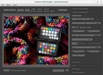
Lumariver Profile Designer, a profile designer based on DCamProf technology. An alternative if you prefer to use a graphical user interface rather than the command line.
Here are the DCamProf downloads:
I have developed DCamProf on Linux and it should be straightforward to build there so I don't provide any Linux binary for download, just get the source and compile.
To build on Windows I recommend MinGW, and on OS X Clang should work, although you need one with OpenMP support. It's a bit more tricky to build on those operating systems, so therefore I've provided separate packages for them that includes just a ready-to-run executable and the documentation. Read the "readme" file first that is in the package.
Graphical user interface
DCamProf is command line software. If you prefer using a graphical user interface I have made a commercial alternative which is built on "DCamProf technology". It's called Lumariver Profile Designer and can be downloaded from www.lumariver.com. It's closed-source and costs money. The sales will indirectly contribute to the DCamProf project which will stay open-source and share core technology with the commercial GUI version.
How DCamProf models cameras
DCamProf looks on the perfect camera as a colorimetric camera, that is the SSFs matches the color matching functions for the CIE XYZ color space. No real camera is colorimetric so the goal of profiling is to make it perform as close as possible to one (and then possibly apply a tone reproduction operator and custom subjective look on top).
DCamProf assumes that the camera is linear, that is if you for example double the intensity of a certain spectrum the raw values will also double and there will be no change in their relation. This is indeed true for any normal digital camera today, with the possible exception of extreme under-exposure and very close to clipping where there can be non-linear effects.
The linearity assumption leads to that the correction lookup table (LUT) only needs to be indexed on chromaticity (that is saturation and hue, but not lightness), but the output still needs correction factors for all three dimensions as some colors can be rendered too dark or too light with a fixed factor throughout the full lightness range. That is DCamProf works with a LUT with 2D input and 3D output, commonly referred to as a 2.5D LUT.
DCamProf does allow you to apply a subjective look on top of the accurate colorimetric 2.5D profile. It will then use a full 3D LUT so you can make lightness-dependent adjustments, but the colorimetric part always stays 2.5D (well, except for some gamut compression of extreme colors, but that doesn't turn up in normal images).
2.5D vs 3D LUT
With a 2.5D LUT we assume that the same color in a darker shade will have the same shape of its spectrum, only scaled down. This is true if you render colors darker by reducing the camera exposure in a fixed condition. However, if we compare a dark and light color of the same hue and saturation in a printed media the spectrum shapes can differ because a typical print technology will alter the colorant mix (eg inks) depending on lightness. In some cases lightness is controlled by adding a spectrally flat white or black colorant, and in those cases spectrum shapes are retained, but that is not always the case.
This means that our linearity assumption breaks as the relative mix of camera raw values may differ slightly between dark and light colors and in this case a full 3D LUT could make a more exact correction. However, this only makes sense in highly controlled conditions when copying known media (such as printed photographs), that is when you're using the camera just like a flatbed scanner. The light source must be fixed, the camera exposure must be fixed, and the camera profile must be designed using a target made with the same materials as the objects you shoot.
As a 3D LUT only makes sense in this very narrow use case DCamProf supports only 2.5D for the colorimetric part (so far). If you really need a 3D LUT you can use Argyll, but you're then limited to ICC profiles. For strict reproduction work that may be a better approach.
Note that commercial raw converters often use 3D LUTs, not to achieve better colorimetric accuracy though but to make subjective "look" adjustments, which you also can do with DCamProf with its "look operator" functionality.
Basic workflow for making a DNG profile using a test target
- Get or make a physical test target. The classic Macbeth/X-Rite 24 patch color checker is a fine choice.
- Get or make a reference file for the
test target, preferably containing reflectance spectra.
- If you're using that 24 patch color checker like most will be doing, the reference file with reflectance spectra assembled by BabelColor is the second best choice if you can't measure it yourself. This data should be valid for the nowadays more popular "ColorChecker Passport" product too.
- The above BabelColor CGATS text file example needs some
conversion to be used with Argyll. To save you some time I've
done it for you, look for
cc24_ref.ciein the DCamProf distribution. - Note that X-Rite changed their formula slightly in
ColorCheckers produced November 2014 and later. The
bundled
cc24_ref.cieis for targets produced before November 2014, andcc24_ref-new.cieis for targets produced November 2014 and later.
- Shoot your test target under the desired light source. Store in raw format.
- Convert the raw file to a 16 bit linear TIFF without white
balancing.
- You can use a recent version of RawTherapee (export for
profiling, with disabled white balance),
or DCRaw
dcraw -v -r 1 1 1 1 -o 0 -H 0 -T -6 -W -g 1
          1 <rawfile>
- If you have an odd camera format and you want to use the profile in Adobe's products it may be safer to convert to DNG first using Adobe's DNG converter, as raw decoding of proprietary formats may differ a little concerning application of black levels, white levels and calibration data.
- Crop so only the target is visible, and rotate if needed. Argyll is very sensitive to target orientation. If you use some image editor to do this make sure that the full 16 bit range is kept, that is don't use 8 bit Gimp for example. If you use RawTherapee you can crop and rotate in there.
- You can use a recent version of RawTherapee (export for
profiling, with disabled white balance),
or DCRaw
- Use Argyll
scanincommand to generate a.ti3file.- It needs the target reference file, test target layout file and raw image as 16 bit TIFF as input.
scanin -v -p -dipn rawfile.tif ColorChecker.cht cc24_ref.cie- Passport version:
scanin -v -p -dipn rawfile.tif ColorCheckerPassport.cht cc24_ref.cie - The
scanincommand will generate adiag.tifwhich shows patch matching (look at it to see that it matched) and arawfile.ti3file which contains the raw values read fromrawfile.tiftogether with reference data from thecc24_ref.ciefile.
- Use DCamProf to make a profile from Argyll's
rawfile.ti3target file.dcamprof make-profile -g cc24-layout.json rawfile.ti3 profile.json- The above command doesn't specify any illuminants, which
means that the profile will be made for D50 and the
rawfile.ti3must contain reflectance spectra (it will if the examplecc24_ref.cieis used) or have it's XYZ values related to D50. To change calibration illuminant use the-iparameter, and if the.ti3lacks reflectance spectra specify its XYZ illuminant using-I. - Per default DCamProf will automatically relax the LUT a bit, that is prioritize smoothness over accuracy. How this is done can be precisely manually controlled if you desire, see the documentation for the make-profile command for an in-depth explanation.
- The target layout is provided in a JSON
file
cc24-layout.json. If the target contains both black and white patches glare will be modeled and reduced, and if the target contains several white patches (not the CC24, but for example a ColorChecker SG) it will be flatfield corrected.
- Convert the native format profile to a DNG profile (DCP).
dcamprof make-dcp -n "Camera manufacturer and model" -d "My Profile" profile.json profile.dcp- For many raw converters the camera manufacturer and model must exactly match what the raw converter is expecting. For example if using Adobe Lightroom the name must match the name Lightroom is using for it's own DCPs.
- The description tag (set by
-d, "My Profile" in this example) will be the one shown in the profile select box in for example Adobe Lightroom. - The above example makes a colorimetric profile without a
curve. If you want to embed a tone-curve and make use of
DCamProf's neutral tone reproduction (which really makes more
sense for a general purpose profile), you can do like this:
dcamprof make-dcp -n "Camera manufacturer and model" -d
              "My Profile" -t acr profile.json profile.dcp
- The DNG profile is now ready to use in your raw converter.
Basic workflow for making an ICC profile using a test target
Making an ICC profile is almost the same as a DNG profile. Actually you can follow the exact same workflow and run the make-icc command at the end instead of the make-dcp, as the native profile format can be converted to both types. However, some raw converters using ICC profiles apply some sort of pre-processing such as a curve before the ICC profile is applied which much be taken into account. Capture One is one such raw converter.
The steps that are the same as in the DNG profile case are only briefly described here, so look there if you need further details.
- Get a physical target with reference file, and shoot a raw file in desired light.
- Export to a tiff for profiling in the raw converter you will be using.
- How you do it varies depending on raw converter, look in its
documentation or search on the 'net.
- Capture One: Select ICC profile: "Phase One Effects: No Color Correction", Select Curve: "Linear Response" (or similar), rotate/crop to show only the target. Then Export variants, "16 bit TIFF", "Embed camera profile". Note: you probably don't want to use "Linear Scientific" as it is a special mode which disables highlight reconstruction. Of course there should be no clipping in the profiling TIFF, but as the profile should be used with the same curve when finished the "Linear Response" is better for all-around use.
- White balance setting does not matter, unless you intend to let the profile correct a camera preset (not a common use case, see make-icc reference documentation for more information).
- If you can choose a curve, choose linear.
- DCamProf must somehow be able to calculate the linear data. If the exported TIFF contains a transfer function tag, like from Capture One, the curve choice doesn't really matter as it can be linearized anyway. I still recommend using a linear curve during profiling, to maximize precision.
- If the exported TIFF doesn't contain a transfer function tag, you should export with a linear curve, unless if you can find out the transfer function in some other way. Note that "linear" doesn't necessarily mean exactly linear in many raw converters so you may need to find out the transfer function anyway.
- How you do it varies depending on raw converter, look in its
documentation or search on the 'net.
- Use Argyll
scanincommand to generate a.ti3file (using the matching.chtfile).scanin -p -v -dipn target.tif ColorChecker.cht cc24_ref.cie- Passport version:
scanin -p -v -dipn target.tif ColorCheckerPassport.cht cc24_ref.cie
- If the raw converter applies a pre-processing curve (like
Capture One), re-process the
.ti3file to get linear RGB data.dcamprof make-target -X -f target.tif -p target.ti3 new-target.ti3- DCamProf gets the pre-process curve from the transfer function tag in the profiling tiff. You can also extract it separately with the tiff-tf command, but as the make-target command can handle the tiff directly it's generally not needed.
- If pre-processing curve cannot be had from the tiff, you
need to supply it in a JSON file (still
-fparameter), see the bundled data example for formatting.
- Use DCamProf to make a native profile from the linear
.ti3file.dcamprof make-profile -g cc24-layout.json new-target.ti3 profile.json
- Convert the native format profile to an ICC profile.
- If pre-processing curve was used it must be given:
dcamprof make-icc -n "Camera manufacturer and model" -f
              target.tif profile.json profile.icc
- ...otherwise the
-fparameter is skipped:dcamprof make-icc -n "Camera manufacturer and model" profile.json profile.icc
- If you want to embed a tone curve and make use DCamProf's neutral
tone reproduction you do like this (both with and without
pre-processing shown):
dcamprof make-icc -n "Camera manufacturer and model" -f
              target.tif -t acr profile.json profile.icc
dcamprof make-icc -n "Camera manufacturer and model" -t acr profile.json profile.icc- The
-t acrparameter will apply Adobe's standard film curve, you can also design your own, or import via the tiff-tf command. - The curve will be applied to the profile's LUT.
- If you're using Capture One, read the section about Capture One and curves.
- If pre-processing curve was used it must be given:
- The ICC profile is now ready to use in your raw converter.
Note that some ICC raw converters do additional processing than just a curve and white-balance, they may for example do some sort of pre-matrixing. If the stripped profiling tiff looks much more saturated than a corresponding tiff from a DCRaw or a DNG profiling workflow it's likely that some pre-matrixing has been applied. As you profile based on the raw converter's own profiling TIFF this doesn't matter, except that the native format profile generated in the process will not be compatible with any other raw converter.
There are also ICC raw converters that do no specific pre-processing, that is provide the ICC profile with "pure" raw input just like to a DNG profile, meaning that you can use the same native profile produced in a DNG workflow and make an ICC profile too. DxO Optics is one such raw converter.
Capture One and curves
Some raw converters allows choosing the curve separately, and Capture One is one of them. This is actually against the design principles used in DCamProf. With DCamProf the profile itself applies the curve partly or entirely via a LUT, and if you want different curves you simply render different profiles, one for each curve. This is because tone curves can fundamentally affect color rendition, as described in the tone curves and camera profiles section.
That Capture One doesn't change ICC profile when the curve is switched you could say is broken color science, however due to the mild shape of their curves and that they are applied before the ICC profile the color appearance is not affected that much. Actually they have a mixed approach, some of the curve is applied separately before the ICC and some is applied by the profile's LUT. This mixed approach makes the color appearance more stable between the different curves than it otherwise would have been, but it also makes the result with "Linear Response" far from actual linear.
In any case you can assume that their bundled profiles have been optimized for the default curve and the others will provide somewhat sub-optimal color, or at least less designed color.
If you like your DCamProf profile to work the same way, you do this way:
- Make a profile with the linear response, that is everything in
the standard workflow until you've run the
make-profilecommand. - Export a profiling TIFF one with the "Linear Response" (let's
call it
linear.tif) and the other with the desired curve, usually "Auto" or "Film Standard" (let's call itcurve.tif). - Extract the actual shape of the curve from the TIFF files, using
the tiff-tf command:
dcamprof tiff-tf -f linear.tif curve.tif tone-curve.json- It may warn that the curves don't end at 1.0, don't worry about that. Capture One does that, probably related to having some margin for highlight reconstruction or white balance adjustments. The tiff-tf command will automatically compensate.
- Make a preliminary ICC profile adapted for the curve's
pre-processing, and also apply the tone curve.
dcamprof make-icc -n "Camera manufacturer and model" -f curve.tif -t tone-curve.json profile.json preliminary-profile.icc- As the pre-processing curve and tone curve are the same, they will cancel out and the resulting profile is linear in terms of contrast, but the neutral tone reproduction operator will have done its work with the appropriate curve, so the profile becomes optimized for that.
- Load the preliminary profile and compare with the bundled. Probably the DCamProf profile has lower contrast because the native profile applies some extra contrast in the LUT. Use the curve tool inside Capture One to manually match the contrast. An exact match is not necessary, what you find most pleasing is the best for you.
- Transfer the coordinates from the curve tool to a JSON file
DCamProf can read, let's call it
modifier-curve.json. Find an example below. - Re-run make-icc with the extra curve cascaded.
dcamprof make-icc -n "Camera manufacturer and model" -f curve.tif -t tone-curve.json -t modifier-curve.json profile.json profile.icc
- The profile is now ready to use. The look will be optimized for the chosen curve, but it will look okay too for "Linear Response", just like Capture One's bundled profiles. Of course, there will be the residual curve left (the modifier-curve) when you use the profile in "Linear Response" mode, in the same way as native profiles.
The modifier curve is suitably designed with the curve tool inside Capture One. Load the preliminary profile generated in the workflow above, and then edit a curve to your liking. Then copy the handle values into a text file with the JSON tone curve format, like this:
{
    "CurveType": "Spline",
    "CurveHandles": [
      [ 0,0 ],
      [ 14,8 ],
      [ 27,20 ],
      [ 115, 118 ],
      [ 229, 233 ],
      [ 255, 255 ]
    ],
    "CurveMax": 255,
    "CurveGamma": 1.8
}
Capture One uses 0 – 255 as their range in the curve, and the curve works with gamma 1.8.
Basic workflow for making a profile from camera SSFs
If you have the camera's spectral sensitivity functions you can skip the target shooting process.
- Format your camera's SSF data into a JSON file that DCamProf can
read.
- Use the distributed examples as a guide for how the JSON file should be formatted.
- If you don't have the equipment or knowledge to measure your camera's SSFs, you can look in the SSF links section and see if you're lucky and can find your camera in one of the sources.
- Generate a "virtual" target with your desired spectral data.
- You can use DCamProf's built-in spectral database or
use its ability to generate spectra, or import from some other
spectral source (see provided
import_spectra.txtfor formatting, it's the Argyll.ti3format, but you can use a subset). - Here's a basic example where we just generate a color checker
from the built-in spectral database target:
dcamprof make-target -c ssf.json -p cc24 target.ti3
- The resulting
target.ti3contains reflectance spectra for all patches, plus XYZ reference values and RGB values for the camera rendered using the SSFs found inssf.json.
- You can use DCamProf's built-in spectral database or
use its ability to generate spectra, or import from some other
spectral source (see provided
- Make the profile
dcamprof make-profile -c ssf.json target.ti3 profile.json- We don't really need to provide the camera's SSF again
(
ssf.json) as the target file already contains rendered RGB and XYZ values, but it's a good habit since then the RGB (and XYZ) values will be regenerated from spectra each time which is convenient and reduces the risk of making mistakes. - If the SSFs are of high quality you will typically get a considerably better match with this than if you have shot a test target. This means that there is often less need of weighting and LUT relaxation when rendering the profile.
- Convert the native profile to a DNG profile or an ICC profile.
- See the description for the basic workflow using a test target for more details.
In this example workflow we keep the illuminants at default, D50. As we let the spectral information follow through in the workflow we can change calibration illuminant late in the process, when making the profile:
dcamprof make-profile -c ssf.json -i StdA target.ti3 profile.json
Note that as SSFs are generally measured from real raw data without pre-processing, profiles generated from SSFs won't work for ICC raw converters that does pre-processing before applying the ICC, such as Capture One.
Choosing test target
Due to natural limitations of camera profiling precision it's quite hard to improve on the classic 24 patch Macbeth color checker when it comes to making profiles for all-around use. It's more important to have a good reference measurement of the test target than to have many patches. If you don't believe me please feel free to make your own experiments with DCamProf; by using camera SSFs you can simulate profiling with both few and many patches and compare target matching between them.
DCamProf allows you to use any target you like though, you can even print your own and use a spectrometer and Argyll to get reference values. Although darker repeats of colors does not hurt there's not much gain from it as the LUT is 2.5D, so an IT-8 style target layout (many patches are just repeats in darker shades) does not make that much sense.
Dark patches are problematic as they are more sensitive to glare and noise (both in camera and spectrometer measurement), so an ideal target has as light colors as possible for a given chromaticity.
The profiling process requires at least one white (or neutral gray) patch, but it tolerates if it's slightly off-white. The target should preferably also contain one black patch which should be the darkest patch in the target. This black patch is used to monitor glare. If feasible the "black" should be made as light as possible while darker than the darkest colored patch. If the black patch is significantly darker than the darkest colored patch DCamProf may detect a glare issue than in actuality only affects the black patch.
The white (and black) patches should preferably have a very flat spectral reflectance, as it makes glare monitoring more accurate.
Most targets have a gray scale step wedge which can be used for linearization. Digital cameras have linear sensors, but the linearity can be hurt by glare (and flare). Normally it's much better to reduce glare to a minimum during shooting than trying to linearize afterwards, as glare distortion is a more complex process than just affecting linearity.
In addition to compensate glare effects DCamProf also has support for flatfield correction which means that uneven lighting can be compensated for. In order to do so you either need a target sprinkled evenly with white patches, or you shoot a separate flat field shot of a completely white chart under the same light. You can read more about this in the testchart-ff command documentation.
(Semi-)glossy targets, such as X-Rite's ColorChecker SG, are extremely glare-prone and therefore hard to use. They cannot be shot outdoors, but must be shot indoor in a pitch-dark room with controlled light. Due to their difficulty during measurement the end result is often a worse profile than using a matte target. Thus I recommend to first get good results with a matte target before starting to experiment with a semi-glossy. Those targets often receive bad reviews simply because the users have not minimized glare when shooting them.
A note about X-Rite targets: due to regulatory and compliance reasons the colors where changed slightly in November 2014, so all targets produced in November 2014 and later has slightly different colors than those produced earlier. This means that if you don't measure your target yourself you need to make sure you have a reference file that matches the production date of your target (DCamProf comes with reference files for both the old and new versions). These things can happen also for other manufacturers and they may not always be announced.
If you have the camera's SSFs you can use the built-in spectral databases (or import your own) rather than shooting real test targets. In that case you will probably want to select spectral data that matches what you are going to shoot, for example reflectance spectra from nature if you are a landscape photographer.
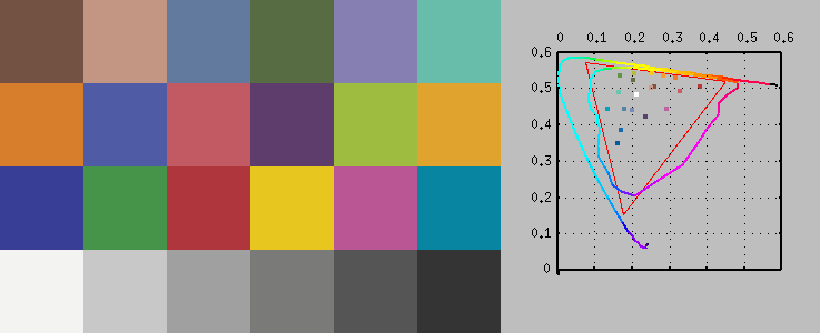
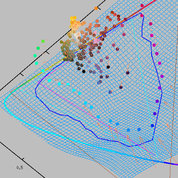
The classic 24 patch Macbeth color checker, originally devised in the 1970's. Despite its age it still holds up well for designing profiles, thanks to relatively saturated colors with a relatively large spread. As seen in the u'v' chromaticity diagram (with locus, AdobeRGB and Pointer's gamut) there's still space to fill though, and some patches are occupying almost the same chromaticity coordinate which is not that useful when making 2.5D LUTs.
Making your own target
Using the make-testchart command you can make your own
target. Here's an example workflow, showing how to make a target for
an A4 sheet and using a Colormunki Photo spectrometer for scanning the
patches:
- Generate test patches in Argyll's
.ti1format:dcamprof make-testchart -l 15 -d 14.5,12.3 -O -p 210 target.ti1- In the above example we specify the chart layout
with
-l,-dand-Oparameters, so that white patches can be placed optimally for flatfield correction later on. The layout must match what Argyll'sprinttargis going to generate.
- Generate a .tif for printing, a .cht file for chart recognition
and .ti2 file for scanning using Argyll's
printtargcommand:printtarg -v -S -iCM -h -r -T300 -p A4 target- It's important that we use the
-rflag, otherwise Argyll will randomize the patch positions which can break flatfield correction. - In the above command we choose A4 sheet and Colormunki half-size patches, it will make 210 patches in one sheet, like we have generated. Even if you don't have a Colormunki instrument the generated patch size is suitable for a test chart for photography (printer profiling targets often have very small patches).
- Print the tiff file on an OBA-free paper matte or semi-gloss, with color management disabled, that is the same way you would print a test chart for printer profiling.
- Measure the reflectance spectra of the patches (this will make a
.ti3file):chartread -v -H -T0.4 target
- Convert the
.ti3to a reference .cie file to be used with Argyll'sscaninlater.spec2cie -v -i D50 target.ti3 target.cie
- Now you have the printed test chart, a
target.chtchart recognition file and atarget.ciereference spectra file which can be used in the profiling workflows.
The quality of your own target will depend on the spectral qualities of your printer. A modern inkjet printer with several inks will have better spectral qualities than many other print technologies, but will still not be as good as the special print techniques used when commercial test targets are made. If you are curious about target performance you can use the SSF functionality of DCamProf to make simulations. Despite spectral limitations it seems that they perform at least as good as a CC24 or sometimes even better when it comes to making profiles that matches real colors.
Semi-gloss targets will get very high saturation patches, but those are difficult for the camera to match and it's hard to shoot those targets without glare issues. They may also be harder to measure accurately with the spectrometer if it has limited range (some consumer spectrometers start at 420nm) or issues with glare. Making a matte target may be better in practice, although you can't get deep violet colors in those.
Test target reference files
The foundation of profiling using test targets is that the profiling software knows what CIE XYZ coordinate each color patch corresponds to, or even better which reflectance spectrum each color patch has so the software can calculate the XYZ values itself.
Higher end test targets may be individually measured so you get a
CGATS text file with reference values, and Argyll's scanin
tool can use them directly. If you get a standard 24 patch Macbeth
color checker you probably don't have an individual reference file and
then a generic file like the one provided with DCamProf will have to do
(cc24_ref.cie for targets produced before November
2014, cc24_ref-new.cie for newer). Having
the reflectance spectra is strongly preferred over pre-calculated XYZ
values, so do get that if you can.
The problem with pre-calculated values and no spectra is that when changing illuminants the software cannot re-calculate XYZ from scratch using spectral data, but must rely on a chromatic adaptation transform which is less exact. It's also a higher risk for the user to mess up by forgetting to inform DCamProf of which illuminant the XYZ values are related to. If there's spectral data the reference values are always re-generated from scratch to fit the currently used illuminant, which is both exact and convenient.
If you have a spectrometer (usually designed for printer profiling) you can measure your target and generate your own reference file with spectra. Using Argyll you do like this:
- Create or find an Argyll .ti2 text file which contains the test
target layout needed for the spectrometer scan. Note that Argyll is
distributed with .ti2 files for many of the popular commercial test
targets, the file is called
ColorChecker.ti2for the CC24. - Scan the target with Argyll's
chartread(exclude the .ti2 suffix, for most Argyll commands the suffix should be excluded):chartread -v -H target- Note that some targets may have too small patches to be read successfully with your instrument. For example an X-Rite ColorChecker Passport cannot be read by an X-Rite Colormunki spectrometer.
- Convert the resulting
.ti3file (which contains complete spectra for each patch) to a new.ti3file with reference CIE XYZ values with your desired illuminant.spec2cie -v -i D65 target.ti3 reference.cie- In the above example "D65" was chosen, but you can also
choose "A" or "D50", or any other supported by the
spec2cietool. - As the spectral data will be kept in the file it actually doesn't matter what illuminant (or observer) you use, you can change that again when generating the profile with DCamProf. The described method is however also compatible with a standard Argyll workflow.
- The resulting
reference.ciecan now be used together with Argyll'sscanintool. - If you don't have a usable .cht file for the chart
layout (a more detailed layout information than needed for the
spectrometer scan), you need to generate one. If you have generated
your own chart using Argyll's
printtargyou can add the-s(or-S) parameter to it to get the .cht file. If you haven't used printtarg it's unfortunately a bit of a headache to make your own .cht. You can use thescanintool as a help for that (using the-gparameter), but it's quite messy with lots of manual edits. At the time of writing I have not tried doing it myself and as long as you're using a reasonable popular target there will be a .cht file distributed with Argyll, and if you make your own using Argyll you can make the .cht when callingprinttarg.
It's probably better to measure your own target and get full spectral information than getting a typical pre-generated reference file with only XYZ values for some pre-defined illuminant. If it really is better depends on the precision of your instrument, the sample-to-sample variation of test targets and the quality of the provided reference file. It's not possible to really know what will be best, you can try both and see what you like the most. If there's some serious problem with the reference file it's usually noticed when making the profile, such as that the LUT must make extreme stretches to match the target or other types of matching issues.
In some cases you may get the reference spectra in some format that
Argyll can't read directly. Argyll is delivered with a few conversion
tools to handle other common text
formats, cb2ti3, kodak2ti3 and txt2ti3. You
may also be helped by making a dummy conversion using DCamProf, like
this: dcamprof make-target -p input.txt -a "name"
output.ti3, and sometimes you must also make some manual
edits in a text editor to get it into a format Argyll accepts.
Shooting test targets
To consider:
- Even light from the desired illuminant, or prepare for flatfield correction.
- Avoid reflections and glare on the target (which is difficult with glossy and semi-glossy targets).
- Avoid colored reflections from nearby surfaces.
- Minimize vignetting.
- Minimize perspective distortion.
- Avoid over- or under-exposure.
Avoid reflections from nearby colored surfaces that may distort the color of the light source. If shooting outdoor, shooting in an open space with someone holding up the test target in front away from the body is a good alternative.
I recommend to defocus very slightly so you won't capture any structure of the target patches surface and instead get fields of pure color. If your camera lacks anti-alias filter this also makes sure you get no color aliasing issues. Shoot at a typical quite small aperture, say f/8 if using a 135 full-frame camera.
Argyll's scanin is sensitive to perspective distortion, so
try to shoot as straight on as possible, and correct any residual
rotation/perspective distortions in the raw conversion. It can
compensate itself using the -p parameter, but it's still
wise not trying to push it.
If you know what you are doing you can push the exposure a little extra to get optimal "expose to the right" (ETTR) and thus as low noise as possible. But be careful, clipped colors will be a disaster in terms of results. I use to exposure bracket a few shots and check the levels in the linear raw conversion to see that there is no clipping. Note that if you're making an ICC profile and use a raw converter that pre-process the raw data with a curve that compress highlights, like Capture One, ETTR is not optimal as that will put highlights in the compressed range. If so expose a bit lower (for Capture One putting the white at about 240 is suitable).
Uneven lighting is a common problem in camera profiling. The typical recommendation is to make sure you have even lighting (at least two lights if not shooting outdoors) and shoot the target small in the center (to minimize vignetting). However, if you employ DCamProf's flatfield correction (the testchart-ff command) you can relax the requirement on even lighting quite a bit. Flatfield correction evens out the light with high accuracy, so you need only make sure all parts of the target has sufficient light to avoid noisy patches. Note that some halogen lights may have an outer rim of light of a different light temperature, and this is not well corrected with flatfield correction. So make sure the target is at least lit with the same light spectrum all over.
Using fewer lights (maybe only one) and compensate with flatfield correction can be a smart strategy when shooting glossy targets, as it's easier to keep the rest of the room dark. Room darkness is very important to reduce glare which is a real issue with (semi-)glossy targets.
Glossy and semi-glossy targets allow for higher saturation colors on the patches, but are also more difficult to shoot as they produce glare. Glare is minimized by being in pitch-dark room and having the light(s) outside the "family of angles". If the target is replaced with a mirror you should only barely see the dark room and camera in it, certainly not any lights. Having a long lens narrows down the family of angles, and a projecting light source (like a halogen spotlight) and dark/black cloth around the target makes sure as little stray light as possible bounces around in the room.
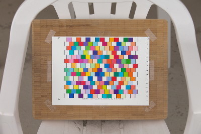
This may look as a perfect target shot, even diffuse outdoor light, no visible reflections. However as the target is semi-glossy the surrounding diffuse light coming from all directions add up the direct reflection component (glare) so the contrast of the target is lowered and the photograph will not match reflectance spectra measurements. Semi-glossy targets must be shoot in indoor lab setups with dark surroundings and projecting light(s) outside the family of angles.
(Semi-)glossy targets are virtually impossible to shot accurately outdoor as you cannot shoot from a dark position, that is if you put a mirror where the target is you will likely clearly see the camera and yourself, which means you will have glare. If you still shoot it in that light it will be affected by glare and produce a lower contrast result, the dynamic range easily drops from 7 stops (typical range in a semi-glossy target) to about half. This won't be visible until you make side-by-side comparison or note poor profiling results (typically an over-saturated profile with some bad non-linearities).
Veiling glare is a lens limitation of how large dynamic range it can capture. It's typically between 0.3% to 0.5% for high quality lenses; the fewer lens elements and better quality coating the lower veiling glare. I mention it here as you may have heard of it, but compared to other forms of glare this is negligible so you don't need to worry about it. Do avoid lens flare though, so the lens front element must be shadowed. Use a lens hood and make sure you have no light sources towards the camera. If you use an SLR camera also make sure the viewfinder is closed tight so no light comes in that way.
If you shoot a glossy target be prepared that you can have issues with dark patches, as those are affected most by glare. Removing those from the measurement (using an exclude list to the make-profile command for example) can be a better way to solve the problem than trying to correct the measurement error in other ways. Due to the many difficulties with semi-glossy targets I recommend to simultaneously make a profile from a matte target so you have a profile to sanity-check against.
In theory a gray scale step wedge in the target could be used to correct glare. With DCamProf you can enable "glare matching" in the testchart-ff command, or directly in make-profile to compensate glare-induced non-linearity. However, glare distorts more than just linearity and in unpredictable ways meaning that any linearization or glare matching will only help to some extent, so don't rely on it. You can indeed improve results this way, but for a glossy target it often ends up worse than just excluding the darkest patches (those that are most affected by glare). So my recommendation is to reduce glare to a minimum when shooting, and keep an extra eye on the performance of dark patches, and exclude them if they seem problematic.
If you shoot a matte target you won't have the same issues with glare so there you can typically include the darkest patches, but it's still often a good idea to enable glare matching to improve the result, especially if you shoot outdoors where the light is less controlled.
White balance and camera profiles
The white balance setting in your raw converter and your camera profile interacts so before making profiles it's good to have some insight into that.
Both DCPs and ICCs make corrections on white balanced data, that is the raw converter pipeline feeds the profile with a white balanced image. For DCPs it might seem that it doesn't as the "ColorMatrix" work on unbalanced image data (more on that later) but the actual color rendering is decided by the "ForwardMatrix" and the LUT, which both work on the white balanced image.
Naturally this means that in order for the profile to make the
"correct" adjustments it must be used with the exact same white
balance as used during profile design. Which is that? Per default
DCamProf will re-balance the target such that the whitest patch in the
target is considered 100% neutral (real targets usually differ 1-2 DE from perfect), which means that white
balance picker on the most neutral patch is the best balance. Note
that the "most neutral" patch may not necessarily be the lightest patch; if the target
contains a grayscale one of the gray patches could be more neutral,
for a CC24 the second patch in the grayscale row is actually more
neutral that the lightest. If you want to you can manually point out
which patch to use as reference using the -b parameter to
make-profile. You would then typically point out the lightest neutral
patch that most would use their white balance picker on in a raw
converter.
You can also disable using an actual patch from the target as reference
(-B to make-profile). Then DCamProf calculates the
optimal white balance automatically, which is when camera white (raw R=G=B)
matches the calibration illuminant reflected by a 100% perfect white
patch (flat spectrum), which is usually slightly different from the whitest patch in
the target.
In any case the reference will be a picked or calculated white balance, not the "As Shot" camera preset balance (there is an ICC special case though where you can design a profile for a camera white balance preset).
A well-behaved profile, that is one with only small and wide area stretches in the LUT, will be robust against slightly different white balances so it won't matter if you set it a little bit off to get a warmer or cooler look for example. A profile which has strong and very localized stretches (not a good profile!) may make sudden strange color changes when you shift white balance. This is because when you change white balance you apply a cast on all colors, which means that the colors move to other start positions in the LUT, and will get corrections that was intended for other neighboring colors, and if there are strong localized corrections the results can become quite distorted.
Wouldn't it be better if the ideal profile white balance was applied first, then the profile, and then your own user-selected white-balance? Yes, if the illuminant would always be the same as the one used when shooting the target, but if you shoot outdoors that's not the case. And in any case that's not how raw converters work so you can't have it that way even if you'd like it.
The take-away message is that for an ideal profile result you should set the white balance to represent white as good as possible, and if you want to make a creative cast, for example a bluer colder look, you should ideally apply that look on top with other color tools rather than the white balance setting. However, many (most?) raw converters don't make it easy to apply a cool/warm look in a different way than using the white balance setting, so that's what we usually end up doing anyway. If you've made a well-behaved profile (which you should) that should not be any real problem. Yes, profile corrections will not be as exact as when used at its designed white balance, but if you're creating a look that won't matter anyway.
The most robust profile concerning white balance changes is a pure matrix-only profile (no LUT), as it's 100% linear. It doesn't mean that it makes as accurate color at other white balances than it was designed for, but it won't suffer from sudden color changes due to localized LUT effects.
DCP-specific white balance properties
DCPs are a bit special when it comes to white balance, they have a more immediate connection to it than ICC profiles.
The embedded "ColorMatrix" is not used for any color corrections, but to figure out the connection between a camera raw RGB balance (internal white balance multipliers which you usually can find in the EXIF data) and illuminant temperature and tint. When you use the camera's "As Shot" white balance, the raw converter will display the corresponding temperature and tint as calculated via the ColorMatrix. This means that if you change profile to one with a different ColorMatrix the "As Shot" temperature/tint will change even if the multipliers are exactly the same. Ideally the temperature/tint should of course show the "truth", the actual correlated color temperature of the illuminant for that white balance, but it's an approximation that may differ quite much between profiles. For a temperature around 5000K a variation of several hundreds of degrees between two high quality profiles is normal, simply because three distinct RGB channels cannot really say much about the shape of a light spectrum. Naturally a profile is best at estimating temperatures close to the one that was used when the profile was made.
If you instead of using the "As Shot" white balance selects a different one with temperature and tint, the ColorMatrix is used to calculate the corresponding white balance multipliers, at least when it comes to Adobe Lightroom (other raw converters may use a hard-coded white-balance model rather than using the profile-provided ColorMatrix). This means that if you change profile to one with a different ColorMatrix the temp/tint will in this case stay the same but the actual multipliers will change and thus the actual visual appearance, that is you get a shift in white balance.
A DNG profile contains the calibration illuminant as an EXIF lightsource tag, meaning that there is a limited set of pre-defined light sources to choose from. For a single illuminant DNG profile this tag is not used though, so it can be set to any value. If you provide DCamProf with a custom illuminant spectrum during profiling the resulting DCP will contain "Other" as lightsource tag, that is no information of what temperature the profile was designed for, but as it's not used it's not a problem.
However if you don't provide the spectrum and instead provide the completely wrong illuminant, say you shoot the target under Tungsten but say to DCamProf that it's D50, the calculated color matrix will be made against incorrect XYZ reference values and the resulting profile will be bad at estimating light temperatures. For single illuminant profiles that still won't affect the color correction though.
Dual-illuminant profiles is an exception. In that case you have two matrices, usually one for StdA and one for D65. Both these are then used to calculate the temperature and tint, and the derived temperature is then used to mix the two ForwardMatrices, that is if it's exactly between the 6500K of D65 and 2850K of StdA then 50% of each is used. This means that the temperature derivation has some effect on the forward matrix and thus some effect on the color correction. So if you intend to make a dual-illuminant profile it's required to provide a proper EXIF lightsource for each, and for the profile to make accurate temperature estimations the actual lights used during profiling should match the EXIF lightsource temperatures as well as possible. It doesn't have to be exact though as any reasonable camera should have similar matrices over a quite wide temperature range.
Note that a DCP profile cannot be made to "correct" white balance, that is change your "As Shot" white balance multipliers to something else. In some reproduction setups you may want to do that, and for this you need to use an ICC profile instead.
When you make your own profile with DCamProf and use it in Adobe Lightroom for example it's as discussed highly likely that you will get a white balance shift compared to the bundled profile. This doesn't mean that there is something wrong with your profile, but simply that your calibration setup and matrix optimizations did not exactly match Adobe's. If you want to apply your profile that previously used the bundled one with a custom white balance settings this white balance shift can be problematic though. Fortunately it's simple to avoid: just copy the color matrix from the bundled profile, which you can do directly in the make-dcp command. It only removes the white balance shift; as the actual color correction sits in the forward matrix and LUTs, the color matrix change will not affect the color rendition (except for the slight effect caused by the dual-illuminant mixing described separately, but you can safely assume that effect is negligible to the profile's performance).
ICC-specific white balance properties
ICC profiles have unlike DCPs no connection to the raw converter's white balance setting. When DCamProf makes its native profiles it makes both a ColorMatrix and ForwardMatrix, but if you convert to a ICC profile only the ForwardMatrix will be used as it has no element to identify illuminant color temperature as DCPs have.Raw converters that use ICC profiles have some other method than using the profile to figure out a suitable temperature/tint to show in the user interface. Maybe by using hard-coded color matrices or hard-coded preset values, or some other proprietary model.
Normally ICC profiles are designed to not affect the user white balance, so when you change profile to an entirely different one the overall tint will still not change (except for tiny changes related to correction of neutrals). However ICC profiles can change the white balance if designed for that. One application could be to make an ICC profile that changes the camera's "As Shot" white balance to match a specific light source used in a reproduction setup. DCamProf can make such a profile if you instruct it to, as described in the make-icc reference documentation. This feature is unique to ICC, you can't make it with DCP as the DCP design prohibits white balance alterations by the profile.
Color for extreme white balances
Raw converters are designed such that "white" should be white (neutral on the screen, R=G=B), but for extreme color temperatures (candle light, Nordic winter dusk etc) this is not how the eye/brain experiences the scene, white objects will have a tint. To render such cases realistically you will have to adjust the look creatively to taste, as the available color models do not support profiling those situations in any accurate way.
Landscape photography in the snow makes this issue very clear. While the snow is "white", you must often tint it to taste to replicate the eye's experience at the scene.
White balance presets
Cameras have white balance presets such as "daylight", "shade", "flash" etc. These are not standardized in any way so it differs between brands and models exactly which light these presets are calibrated for. That is a white patch that becomes 100% neutral (R=G=B) in a specific light for camera A's daylight white balance setting will have a slight tint for camera B's daylight setting.
If you design two profiles for two different cameras with the exact same target under the exact same light, and you use the white balance picker to set a custom white balance on the white patch, it will be very difficult to tell the two cameras apart, they will look almost exactly the same. However if you usually use a preset on the camera, say the "daylight" preset which is common in landscape photography, it's highly likely that the cameras will have a visible difference in look. For example that one camera will render slightly warmer tones than the other, and this is simply because the white balances are different. In other words profiles can only make two cameras look the same if white balance is tuned for the same white.
Ideally it would exist a profile standard so you could load profiles directly into the camera and re-program the white balance presets. Or even better, profiles would store the SSFs so the raw converter could have its own preset light source spectra and accurately calculate corresponding white balance multipliers for any camera. But this does not exist. So how to relate to what we have got?
First let's consider what the problems are. The main problem is that if you use white balance presets the look will change if you change camera, for example if you make a switch in the middle of a shoot, or if you upgrade to a new camera later. If you always set the white balance with a white balance picker you don't have a problem, the cameras will then produce the same look (assuming both have been profiled in the same conditions).
There's another theoretical problem which is that the profile's LUT expects that white is perfectly neutral as that is the reference point for the non-linear corrections, and if the white is tinted the corrections will be skewed. I say it's theoretical though, as any well-behaving profile makes broad smooth corrections and the error introduced with a white balance offset is considerably smaller than the overall inaccuracies in camera profiling.
However, for completeness let us look at this theoretical problem first. Say if we want to use an in-camera preset and want the profile to be perfectly calibrated for that, then there are two ways. Either you match the illuminant in the target setup with the in-camera preset so the white patch becomes 100% neutral (almost impossible without a programmable spectrum lamp), or you create a new in-camera preset (most cameras allow custom presets) that matches your target setup light. Instead of making a in-camera custom preset you could make a white balance preset in the raw converter.
You could do this, but for general-purpose photography it's way overkill, and often does not make any sense as the actual light used when shooting is probably varying (if you shoot outdoor). The only thing this matching will provide is that if the light you shoot in happen to render neutrals 100% neutral with your preset, then you know that the profile's LUT corrections will be applied as correctly as possible. But even then, it's not certain as you cannot really know if the shape of the illuminant spectrum is matching what you used when shooting the target, and of course the variability of spectral reflectance of different colors come into play too. In short, I hope it's clear that it's not worthwhile to think about that aspect.
Next let's look at the "real" problem, which is matching two different cameras when using white balance presets. The common "solution" is simply not care, let cameras differ and use a white balance picker in cases it's important to match them. Most users are pleased with this approach, and I recommend to do so unless you do have a specific need to match camera presets. However, even if you don't worry about matching cameras you may not like the tint of the built-in presets, maybe they're generating a too warm or too cool look for your typical shooting conditions. In that case you need to make your own custom preset, either in-camera or in the raw converter.
Most raw converters have their own built-in white balance presets, but it differs between them how they are applied. A camera manufacturer's own raw converter probably has the presets matched with the camera so they are the same. Third-party raw converters, like Lightroom, usually have their own fixed presets which don't match the camera's own. Using Lightroom as an example, its "daylight" setting is fixed at 5500/+10 (which by DNG/Adobe definition matches D55) and it uses the profile's matrices to figure out which actual RGB multipliers (raw white balance) that temperature/tint setting corresponds to. Will camera A and B match if using those presets? Maybe. If you profiled both cameras in the same setup and the target illuminant was (said to be) D55, then they should match for that setting, but if you change preset to say Shade (7500/+10, D75) the color matrix calculations will most likely be too inexact to make a match. To be fair, to match cameras over several presets you really need to profile each illuminant separately (or measure the SSFs), getting a match at the profiled illuminant is the best we can expect.
So for Lightroom you could profile both cameras under the same light, and tell DCamProf that it is D55 (it doesn't really need to be exactly that), then you can use Lightroom's built-in "daylight" preset and the cameras will match, but only for that preset (and light). The same method may or may not work for other raw converters using DNG profiles, depending on how the white balance handling is implemented there.
The "fool-proof" way is to make a custom preset for each camera based on white-balance picking in a fixed setup. It doesn't need to be your target setup, it can be any situation only if both cameras was shot in the same occasion. It's of course an advantage to use a fixed setup with artifical light as it can then be recreated later when getting additional cameras. A problem here is that you may not have access to a light which gives you a suitable preset, maybe you want the preset to make a warm tone in daylight, and then you need a cooler light to profile for. The solution to this is to use a target which has off-white patches (warm and cool) so you can pick and choose a tint. X-Rite's ColorChecker Passport has such patches.
You can of course also tune your presets "by eye"; pull the sliders until you are satisfied and save it as a preset. If you make the preset in-camera or in the raw converter is a matter of taste (and a matter of how well the camera supports custom presets).
With an ICC profile you can shift the neutral, so instead of making a custom preset in your camera or raw converter you can shift the neutral so the in-camera preset matches your custom white balance. DCamProf can make such profiles. It should be said it's an unusual way to approach the problem though and I don't recommend it for general-purpose profiles. DNG profiles can't shift the neutral axis so it's not possible to use them with this method.
My recommended approach to white balance presets (assuming you like to use them rather than using auto-white balance or picking white balance each time), is to either not care, letting cameras tint the way the manufacturer likes, or make manual presets by tuning by eye to taste. If you intend to leave it alone, still check if you like the tints the camera presets give you, and make custom ones if you don't like them. If you have a real need to match presets of several cameras, the best way is to use a fixed setup with an artificial light as close as possible to your desired light (so you can recall it later when getting additional cameras), and then create custom presets by white balance picking on a target. You could use a target with tinted off-white patches for greater flexibility on choosing if it should render warmer or cooler than the used illuminant.
Tone curves and camera profiles
An example image rendered with a linear tone curve using an accurate colorimetric profile. The exposure has been increased to make the image easier to compare with the others that have tone curves (as the tone curve has a strong brightening component).
This image should be used as reference when evaluating accuracy of colors. However, it does look flatter than the eye experienced in the brighter real scene, which is a normal appearance phenomenon. This means that we need to apply some sort of curve even when we want a neutral realistic look.
Same profile, but now with the DNG default curve, which is a modified RGB curve. Note the garish colors. Light colors are also desaturated, not so easily seen in this picture although the white shirt has lost much of its original slight blue cast. Desaturation issues can more clearly be seen in light blue skies for example.
DNG uses a hue-stabilized RGB curve (constant HSL hue) so it's better at retaining hue than a standard RGB curve (which most ICC-based raw converters use).
Same profile, with the tone curve applied on the luminance channel, while hue and saturation are kept constant. As luminance channel the J of CIECAM02 Jab is used here, similar to the more well-known Lab.
Intuitively one may expect this to be truest to the original, but as seen it looks desaturated. This is because in human vision color appearance is tightly connected to scene contrast, so if you increase contrast also saturation must be increased to maintain the original appearance.
Same profile, here with DCamProf's built-in neutral tone reproduction operator. Color appearance is now very close to the original linear curve, but we have increased the global contrast so the photo displayed on a screen appears truer to the real scene.
Adobe Camera Raw's profile with the intended tone curve (same as in the others). Looks pretty natural, but some issues with saturated colors; too saturated reds and too little saturation on the purple and bright yellow-green. Additionally, skin-tones are slightly over-saturated and yellowish, and again the slight blue tint of the white shirt has been lost.
While some errors can be side effects of the curve, they're mainly deliberate subjective adjustments by Adobe's profile designers with the purpose to achieve a designed "look", like film have in analog photography. DCamProf's tone-curve operator is instead designed to stay true to the color appearance of the original scene and leave subjective adjustments to the photographer.
Adobe Camera Raw's profile with linear tone curve. Here we can clearly see that it's not a "scene-referred" profile. The profile has been adapted for the S-shaped DNG tone curve and is therefore desaturated.
Note that comparing all these pictures may be hard directly on this web page as color shifts slightly with viewing angle. To critically compare, first download the files and then look straight at them while flipping through them in an image viewer. The images were made during development so the result from the current may differ a little, but you should from these images get an idea what the typical differences are and how large they are.
- As soon as you apply a tone curve you significantly alter the look of the colors.
- The well-known raw converters' tone curves don't work well with linear "accurate" profiles, but will produce garish colors.
- Ignoring the effect of tone curves is what makes many self-made profiles fail for all-around use.
- There is no established standard tone curve that produces neutral results as the standard color appearance models like CIECAM02 don't embrace the tone curve concept.
- Applying the curve on the L channel in Lab or V channel in HSV or L in HSL all have problems. For a high end result a custom tone reproduction operator is required.
A linear tone curve is the right thing for reproduction work, for example when we shoot a painted artwork and print on corresponding media. In this case the input "scene" and output media have the same dynamic range and will be displayed in similar conditions. However in general-purpose photography the actual scene has typically considerably higher dynamic range than the output media, that is the distance between the darkest shadow and the brightest highlight is higher than we can reproduce on screen or paper.
The solution to this problem since the early days of photography is to apply an S-shaped tone curve. In analog film the curve compresses highlights and shadows about equal (a sigmoid curve), while in digital photography there's been a shift to compress highlights more than shadows, which also brightens the image about a stop or so as a side effect. This suits digital cameras better as it retains more highlight detail. The principle is the same though, that is increased slope at the midtones with compressed shadows and highlights.
The need to compress highlights and shadows is obvious (otherwise we would not fit the scene's original range on the lower dynamic range available on screen), but do we really need to increase midtone contrast? The usual explanation is that the output media has lower contrast than the real scene and thus we need to compensate to restore original contrast. While this can be said to be true for matte paper, a calibrated screen will produce appropriate contrast for midtones. It surely cannot shine as bright as the sun and (probably) not make shadows as dark as in real life, but midtone contrast is accurate. In typical workflows we adapt the image first for the screen and then make further adaptations for prints (screen to print matching is a separate and well-documented subject), so when it comes to camera profiles comparing with screen output makes most sense which we will do here.
If we increase the midtone contrast with our tone curve, we will exaggerate. For a typical curve type this is mainly seen as increased saturation, as increased contrast separates the color channels more which leads to more saturation. Okay, so this is wrong then? Well, it's not that simple. Let's say we display a shot of a sunny outdoor scene. Although midtone contrast on the screen can be rendered correctly, the overall luminance is much lower. This makes the Stevens and Hunt color appearance phenomena come into play, that is the brighter a scene is the more colorful (=saturated) and contrasty it appears. That is to make the displayed photo appear closer to the real scene we need to increase both lightness contrast and colorfulness, which an S-shaped tone curve does for us.
So then all is good with the tone curves applied by typical raw converters? No. In fact if we're into a neutral and realistic starting point it's not good at all. Most converters apply a pure RGB curve which has little to do with perceptual accuracy. Lightroom and many DNG raw converters apply a slightly different RGB curve that reduces hue shift problems (HSV hue is kept constant), but it's still in most situations almost identical in look to a pure RGB curve. It varies between converters in which RGB space this curve is applied, which also affects the result. In Lightroom/DNG it's always applied in the huge linear ProPhoto color space, while in many ICC raw converters it's applied in a smaller color space.
Let's start with the RGB tone curve problems. It will increase saturation more than is reasonable to compensate for Stevens and Hunt effects, so you get a saturated look. You might like that, but it's not realistic. Another problem is that for highly saturated colors one or more channels may reach into the compressed sections in highlights or shadows and that leads to a non-linear change of color, that is you get a hue shift. Typically the desired lightening and desaturation effect (transition into clipping) masks the hue shift so it's not a huge problem, but it's there.
Then there is the color space problem. If the RGB tone curve is applied in a large color space such as one with ProPhoto primaries (like in the DNG case) one or more channels can be pushed outside the output color space (typically sRGB or AdobeRGB) so we get clipping and thus a quite large hue shift. Some raw converters partially repair this through gamut mapping (Lightroom does), but still there may be a residual hue shift.
To battle the various RGB tone curve issues bundled profiles typically have various subjective adjustments to counter curve issues. For example the profile may desaturate high saturation reds to avoid color space clipping. Naturally this means that the same profile used with a linear curve will produce too little saturation in the reds. That is a profile must be specifically designed for the intended curve.
I think this is bad design. In fact one could argue that staying with RGB curves (and similar) has inhibited the development of good profiling tools and makes it unnecessarily hard to get natural colors in our photos.
It doesn't have to be this way, the RGB tone curve is legacy from the 1990s when its low computational cost was one of the reasons to use it. It can also be seen as a nostalgic connection to film photography. In the film days the film had to produce the subjective look too, so exaggerated contrast and saturation were desirable properties. This thinking has been kept in most raw converters today despite that we have all possibilities to start from a neutral look and design our own on top rather than relying on bundled looks. The RGB tone curve produces a saturated look that many like to have in their end result, but as said it still doesn't work well for profiles that aren't specifically adapted for it.
Using a DCamProf neutral linear profile and applying and RGB tone curve will produce a garish look. As we will see, the solution to this problem is to use DCamProf's built-in neutral tone reproduction operator.
Tone reproduction operators
In the research world the problem of mapping colorimetric values from a real scene to the limited dynamic range on a screen or print is well-known and is the subject for many scientific papers. The scientific term for the "tone curve" that compresses the dynamic range to fit is "tone reproduction operator", and can instead of a simple global tone curve be scene-dependent and spatially varying, what we in the photography world call "tone mapping".
In science the goal is generally to make an as exact appearance match as possible, for example if we have shot a scene in very low luminance level (at night) also the eye's night vision with its limited ability to register color is modeled. Modeling all aspects of human vision at the scene and at reproduction is a complex problem and is still a very active area of research.
Current raw converters are not designed for this type of advanced appearance modeling and it's generally not what a creative photographer is interested in. For example, in night photography we typically want to make use of the camera's ability to "see" more saturated colors than our eye can.
There is a middle way though. While we do want to increase contrast and don't really mind that it will be more than realistic for scenes not shot in bright sunlight, RGB tone curve color shifts are not beneficial. That is the tone reproduction operator we want for general-purpose photography is a basic S-shaped tone curve just like in traditional photography but without color shifts. This middle way has not got much attention in the research world though. Once computers got powerful enough researchers moved away from the "simple" tone curve models into tone mapping.
While tone mapping is useful in many cases, it's better handled separately in practical photography. It doesn't replace the need of a tone curve-based operator, it's just a complement. Due to the lack of research there is no established operator with the desired properties though, so I had to come up with an own for DCamProf.
DCamProf's neutral tone reproduction operator
With DCamProf I've chosen the approach to render accurate neutral linear profiles (scene-referred), and then develop a new spatially uniform tone reproduction operator that doesn't have the hue shift and over-saturation problems of the commonly used RGB curve. This means that the profile can be developed just like a "reproduction profile" and no subjective tuning is required to adapt for the RGB curve's issues.
This operator can be applied when generating a DCP or ICC profile so you can achieve the intended look in your raw converter.
It has the following properties:
- Luminance is the same as a DCP tone curve applied in linear
ProPhoto space
- This means that the contrast and brightening will be the same as a standard DCP/RGB curve, so you can use the same curve shape.
- Exception: for high saturation colors (flowers etc) a pure luminance curve is blended in, as it has better tonality.
- The contrast (the curve shape) is a subjective choice made when
generating the profile.
- Typically one chooses a contrast that looks realistic for bright sunny outdoor scenes, and thus exaggerates contrast for other scenes, which generally is desirable in terms of subjective look.
- If we'd want a realistic contrast curve for all types of scenes the curve would have to be scene-specific, and then the raw converter would have to work with linear profiles and apply curve itself. However, most raw converters are designed for profiles that have a fixed curve applied.
- Hue is kept constant.
- Small exceptions to this rule close to clipping in some color ranges to improve smoothness of gradients.
- The contrast of the curve is measured and the saturation is
adapted accordingly so the perceptual impression is that saturation
is kept constant.
- Higher contrast needs higher saturation, otherwise the image would look desaturated.
- Highlights are desaturated (less so than in an RGB tone curve though) to make a nice transition into clipping.
- Non-linear elements are used where it adds perceptual accuracy, but the algorithm has been kept as simple as possible.
- Compared to an RGB tone curve this operator increases saturation less and minimizes hue shifts.
ntro_conf.json file in the data-examples directory
for a documented example (the file contains the default weights).
The operator makes no local adjustments, and as it's just a part of a camera profile it can't do that anyway. This means that only the curve is analyzed for contrast, and as an image can vary in contrast locally (for example a large flat blue sky has low contrast even if the curve is a steep S-curve) also the eye's perception of color vary a little over the image surface, and thus some areas may receive a bit too much saturation or too little. This is not a large problem, but something to be aware of when evaluating results.
DNG profile implementation notes
When making a DNG profile the operator is implemented through the LookTable and curve. So if you strip away the LookTable and curve you have the pure colorimetric profile left.
The DNG profile LUTs are not as flexible as ICC LUTs, most notable is that you cannot alter grays, not increase saturation or change lightness (value). As the LUT works with multipliers on saturation it's logical that you cannot increase saturation from zero. However, it's not logical that value cannot be scaled. Some DNG profile implementations support scaling grays (as the LUT itself does support), but the public DNG reference code as well as Adobe's products ignore the value multipliers for gray and instead set them to 1.0, that is no change.
This means that you cannot implement a curve directly in the LUT, as grays cannot be darkened or brightened (which a curve requires). The workaround is to embed a DNG tone curve (which can scale grays), predict the result of that curve and reverse the undesired effects to get the intended result. This is how DCamProf does it. There is one potential problem though: it's not specified in the DNG specification how the tone curve should work, so there may be raw converters out there that does not use Adobe's hue-stabilized RGB curve variant and if so you will not get the desired output.
If you come across such a raw converter (unlikely) and want to use this tone reproduction operator, please let me know.
(So how does actually Adobe's tone curve work? It's an RGB curve where the tone curve is applied on the largest and smallest value, and then the middle value is adapted to keep a constant hue as defined by RGB-HSL/HSV. In terms of look and saturation increase it's very similar to a pure RGB curve, more so than a HSL-L curve or HSV-V curve, but some color shift problems are avoided.)
The LookTable will in DCamProf's profiles per default be gamma-encoded for the value divisions, this will make perceptually better use of the range (that is higher density in the shadows) meaning that the default 15 value divisions should be enough for most curves. Some older or simpler raw converters may not support the gamma encoding tag though, and if so you can disable it.
In any case will DCamProf's DNG profiles with the neutral tone reproduction operator applied be quite large in size. There is no way around that as the DNG profile format is not designed to be space efficient for profiles that do not embrace Adobe's RGB-centric idea of camera color.
Verifying tone reproduction accuracy
Once you have applied a curve you can no longer do normal automatic delta E comparisons to check for accuracy. By definition a curve adds a lot of lightness "errors" as it applies contrast, and we also add saturation "errors" to perceptually compensate for the increased contrast. The one-to-one delta E comparisons only work for linear profiles.
There are no readily available color science models top help us out here, so the only method at hand is to verify by eye. To do this you make a linear profile that can be measured for accuracy and use that as reference. Then make two copies of each test image, one with the linear reference profile applied, and one with the curve. Then you make A/B swapping to compare these images. It's important to do swapping and let the eye adapt for a couple of seconds, if you would compare side by side the eye will be confused by the two different contrast levels displayed simultaneously.
Check that individual hues seems to be the same and look globally and see if saturation seems to match. If you look closely on one isolated color without seeing the global contrast, saturation should be a little higher for the curve profile.
A photograph with faces in it is one good reference point, as our eyes are very good at detecting subtle differences in skin tones. I also recommend testing a sunny outdoor landscape scene, where you can check if the applied contrast is suitable: look globally and get a feel if the scene looks as contrasty as in real life but without exaggeration. Check if the color of the blue sky seems right, hue shift of light tones is typical for simpler curves.
I also recommend testing a photo with various high saturation colors which you can find in flowers naturally or as artificial colors for example in toys or sports clothing. High saturation testing is a bit difficult as you can run into color space clipping. Using a wide gamut screen will certainly not hurt in this case.
As mentioned in the description of DCamProf's neutral tone reproduction operator camera profiles are limited by that they can only apply a global adjustment, and thus not make any local adjustments adapted specifically for the image content. Keep this in mind when evaluating the result.
Scene-referred versus output-referred
You have probably heard or read that "DNG profiles are scene-referred and ICC profiles are output-referred", and in the next sentence it's said that scene-referred is better. What does this mean?
A scene-referred camera profile simply means that the purpose of the profile is to correct the colors so the output represents a true linear colorimetric measurement of the original scene. In other words we want the XYZ values for the standard observer, or any reversible conversion thereof. That is what we in daily speak would call an accurate linear profile (where linear means "no tone curve", we can still employ a LUT for non-linear correction), which DCamProf makes per default.
An output-referred camera profile should instead produce output that can be directly connected to a screen or printer ICC profile and produce a pleasing output for that media. As discussed, for cameras this means in practice that there should be some sort of tone-curve applied to get a pleasing midtone contrast and compressed highlights. In other words if the camera profile converts to XYZ space, those XYZ values should already have the curve applied and also any other subjective adjustments.
It's true that the ICC standard is written such that it expects camera profiles to work this way. However, raw converters that use ICC profiles don't necessarily follows this intention. Some let the ICC profile make a scene-referred conversion, while some makes some sort of mix between scene-referred and output-referred (let it do subjective color adjustments, but not apply a curve), and only a few do it the ICC standard way and make the ICC profile fully output-referred.
While DNG profiles can be 100% scene-referred, they can also have a "LookTable" LUT and/or a tone curve which are subjective adjustments for output, effectively making the profile output-referred. Adobe's own profiles have these type of adjustments, and are thus output-referred.
Due to these variations of how the profile formats are used I think the scene-referred versus output-referred discussion is a bit confusing. DNG profiles supports both things natively and ICC profiles do it in practice depending on raw converter design.
To support all-around use of scene-referred profiles the raw converter must have a type of tone reproduction operator that can change contrast without distorting color, otherwise scene-referred will only make sense with the linear curve. None of the big name raw converters have such an operator but instead require profiles to be adapted for a curve if you want realistic color. This is why DCamProf supports applying its own tone reproduction operator directly in the profile.
Tone curves and matrix-only profiles
To compensate the negative color shift effects of an RGB tone curve the profile needs to make non-linear adjustments. This is not possible with matrix-only profiles as they by nature are 100% linear. However, a matrix profile made to match a matte target, such as the classic CC24, will most likely produce too low saturation of high saturation colors, and will thus produce a less garish look together with an RGB tone curve than a colorimetric LUT profile would (which can accurately reproduce high saturation colors as well).
It's generally not a good idea to try to get good match of high saturation colors for a matrix profile in any case, as that will reduce precision of the more important normal range of colors. That is a good matrix profile is generally a bit desaturated and therefor works okay (although not perceptually accurate) together with an RGB tone curve in most circumstances.
DCamProf does not provide any functionality to adapt matrix-only profiles for tone curves, so if you intend to use your matrix profile with an RGB-like curve make sure you design it with not too high saturation colors.
The look of over-exposure
Digital cameras clip the raw channels straight off when over-exposed which may not result in a pleasing look, even together with a roll-off in the profile's tone curve. To handle this some raw converters renders over-exposed shots differently, to mimic how over-exposed analog film looks, meaning that further lightening and desaturation is applied.
This special rendering mode of over-exposed images is not standardized and cannot be controlled by the camera profile. There should be no need to do so either, but it's good to be aware of this if you compare output of the same camera profile in two different raw converters. If the shot is over-exposed the raw converter itself may affect the look. Naturally if you lower exposure of a clipped image the raw converter's highlight reconstruction algorithm will affect the look, which also is outside the control of a camera profile.
Chromatic adaptation transforms in camera profiling
If the light of a scene changes from say a blueish daylight (D65) to a reddish tungsten (StdA) and we give some time for our eyes to adapt the colors will still look approximately the same. This is the eye's chromatic adaptation, and the phenomenon that colors appears the same when viewed under different lights is called "color constancy".
However, the eye is only approximately color constant, that is some colors will appear slightly different under the new light. In color science the chromatic adaptation behavior of the eye/brain has been tested with various psychophysical experiments where test persons match colors under different lights, in order to find "corresponding color sets". The corresponding color under a different light can be a different sample, which is an example of "color inconstancy".
These experiments have then served as basis when developing chromatic adaptation transforms, CATs, mathematical models of the human vision's chromatic adaptation behavior. A CAT thus models both the color constant and the inconstant parts of adaptation.
A CAT does the following: provided a CIE XYZ tristimulus value under a source illuminant, predict what the XYZ tristimulus value should be under a destination illuminant that provides the same color appearance. The illuminants are given as whitepoints (white as tristimulus values), so the CAT does not need any spectral data.
In camera profiling a chromatic adaptation transform is needed when the calibration illuminant is different from D50. The reason for this is that the profile connection space is always D50 (for both ICC and DNG profiles), that is the color rendering pipeline in raw converters need the profile to output colors relative to D50, which then can be converted further to colors for your screen or printer.
If the profile is made for say tungsten light (StdA, 2850K) we then need to convert those XYZ coordinates to corresponding colors under D50. This can be made with a CAT, and the current best for these tasks is the CAT coming with the CIECAM02: CAT02. However, the CAT is still far from perfect. There are challenges concerning the accuracy of the experimental data they are based on, and the experiments cover only a limited illuminant range (usually StdA to D65) and limited range of colors. In addition are the CATs designed with various trade-offs to make them easier to use mathematically. And finally, these transforms work on tristimulus values only, of both colors and illuminants. Any knowledge of spectral information won't contribute.
"Relighting" transform
There's also another type of chromatic transform which sometimes is needed in camera profiling. Let's say we have the XYZ value under D50 for a test target patch, and we want to predict which XYZ signal we will get from the same patch lit under StdA. That is we're relighting the patch. If we have the reflectance spectrum of the patch and the destination illuminant it's straight-forward: we just calculate the new XYZ values the normal way with spectral integration.
However some reference files provided with commercial test targets only have XYZ coordinates, and if we don't have a spectrometer to measure the target ourselves then we need to make a transform without having any spectra at hand.
This transform is not the same as a CAT. A CAT finds a corresponding color and models the color inconstancy aspects of human vision. However, as human vision is approximately color constant many software applications use a CAT anyway when a relighting transform is called for, and there's not much else to do as the established color appearance models don't provide any other transform. There is no standardized name for the "relighting transform" which means that CAT is sometimes used in the literature also for this which causes some confusion. In this documentation the term "relighting transform" will be used.
With DCamProf there is a better alternative for relighting than using a CAT. If the reflectance spectrum is missing DCamProf can generate a virtual spectrum which matches the given XYZ coordinate, and that spectrum can then be lit by any illuminant. Of course the rendered spectrum will not exactly match the unknown real spectrum, but tests made on various sets show that for most colors this method outperforms both Bradford CAT and CAT02. Rendering virtual spectra often gets you within 1 DE from the correct answer, while the CAT is often in the range 2-4 DE.
Performance of CATs
The performance of a relighting transform is easy to verify as long as you have spectral data, and there are plenty of databases with various spectra to run tests against.
With a CAT the only data to verify against is the correlated color experiments made, and CAT02 generally wins when it comes to the established models. However, as discussed all of these models are rather approximate, and the question arises that maybe they introduce more errors than they fix? A CAT02 conversion from StdA to D65 will have about 3-4 DE on average compared to the correlated color set experiments. Performance is probably not so good outside the StdA to D65 range as the reference experiments don't cover a wider range than that.
It would be most interesting to compare CAT with simple spectral relighting, as the latter is usually available when profiling. When using the relighting transform as a CAT we assume perfect color constancy, which indeed is wrong, but on the other hand the error will be no larger than the range of color inconstancy, which presumably is quite small. Unfortunately the correlated color experiments don't have spectral data so there is no way to make this comparison. What we can see though is that relighting is about 3 DE on average from CAT02, with up to 6-7 in saturated reds and yellow-greens.
From these results a fair guess is that a CAT is indeed better at predicting the color inconstancy aspects of human vision than just keeping perfect color constancy (that is do relighting from spectra), but also that relighting may be more robust and may have smaller appearance errors in some ranges.
When are CATs and relighting used?
If you make a D50 profile and have D50 XYZ target reference values no CAT or relighting is required. If you like you can make a D50 profile even if the actual light used when shooting the target is not D50. What then will happen is that the color appearance will be as if lit by D50, but the profile will only work as intended in the light used at shooting time (if you make a DCP it's light temperature estimation will be off too, but that does not hurt performance in any way).
DCamProf needs target reference values as illuminated by the calibration illuminant (= the light the target was shot under). Why? There are two reasons, one is to calculate the color matrix which is used in DNG profiles to estimate light temperatures, and the other is to know the color appearance under that light so we can using a CAT get corresponding colors for D50, used in the profile connection space where color correction takes place.
The reference file tristimulus values are often calculated for D50 and as soon as our calibration illuminant is different from that a relighting is required. If spectra is available in the target file this is done by spectral calculation which yields accurate results. If spectra is missing a relighting transform has to be applied.
DCamProf also needs D50 reference values, as D50 is the reference in the profile connection space where the color correction matrix (the "forward matrix") and LUT work. If the actual look of the calibration illuminant should be retained we need to model also the color inconsistency aspects of human color vision and then a CAT is used, so we take the reference values calculated for the calibration illuminant and transform those to D50 via a CAT.
With DCamProf you can if you want force color constant behavior and then D50 values will be calculated via relighting rather than a CAT, assuming target spectra is available. If you are making a reproduction profile this is likely what you want.
Note that if we don't make a DNG profile, or we don't care about its ability to estimate light temperatures, and we rather use color constant behavior than using CAT, the reference values for the calibration illuminant will not be used.
Summary:
- For D50 profiles with D50 reference values in the target neither CAT or relighting will be used, as it's not needed. This is the most common use case.
- Relighting is performed to get XYZ reference values for the calibration illuminant (unless the XYZ reference values was already made for the calibration illuminant).
- The (often relighted) calibration illuminant reference values
are used for two things, and depending on context these may or may
not be used in the final profile:
- To derive the "color matrix" used by DNG profiles for light temperature estimation. It's not used by ICC profiles.
- To serve as starting point for the CAT02 transform to D50,
the illuminant for the profile connection space where the color
correction matrix (the "forward matrix") and LUT works, that is
where the actual color correction takes place. If color constant
behavior is enabled (
-Cflag), this case will not be applied.
- If color constant behavior is enabled (
-Cflag), relighting rather than a CAT is used to get the D50 reference values. As reference files typically contain D50 values to start with relighting is often not necessary. - If no spectra is available in the target file and no virtual
spectra is generated, the Bradford CAT is used as a "poor man's"
relighting transform. It's generally better to enable virtual
spectra generation (
-Sflag) in this situation as it provides more accurate results. - Color constant behavior is generally desired in copy applications, while using CAT to model real appearance is typically preferred for general-purpose profiles.
Testing CAT-designed profiles
If a CAT was employed when designing the profile, for example to keep
the color appearance of colors under tungsten light, you should test
the profile with the same criteria. Using DCamProf's test-profile
command you can just mirror the parameters from make-profile. If you
use some external software for testing it's likely that it will not
apply a CAT and instead expect perfect color constancy. In that case
you should either not use that software for testing, or redesign your
profile with the -C flag, that is disable CAT.
Subjective looks in camera profiles
The camera profiles bundled with the big name commercial raw converters are generally not designed to reproduce accurate colors, but instead apply a more or less subtle designed subjective look. The central aspect is the tone curve, as discussed separately in the tone curve section, but the appearance of colors are also adjusted with the intention to produce a more "pleasing" result than an accurate profile would. For example a profile may render smoother and less reddish caucasian skin-tones for flattering portraits, and more saturated colors overall to make landscape images "pop".
This is very similar to how color films worked — few aimed for accuracy but instead different types of subjective color that could suit more or less well depending on subject. Contrast (tone curve) differed between films too. It could be said that today's digital camera profiles builds on the film tradition. Although we with digital technology could design the look separate from the profile (using the raw converter adjustments, or a photo editor), the traditional way with preset looks is still alive and well.
These subjective profiles can be arranged for use in the raw converter in various ways. Some concepts may be found in several raw converters, and others are more rare.
The illuminant selection (typically tungsten, flash and daylight) is not about subjectivity but about adapting the camera response to a light source, it's still often a part of the profile choice unless it's automatically derived from the white balance setting. Dual-illuminant DNG profiles have it built-in, and also some proprietary profile formats. Many raw converters that use ICC profiles allows some sort of illuminant choice, assuming that the manufacturer have spent effort making profiles for several illuminants.
Then there's often a choice depending on intended subject, such as "portrait", "product" and "landscape" which are true subjective looks with specific color adjustments to make flattering and pleasing images for the intended subjects. Sometimes the tone curve is integrated into the profile (lower contrast for portrait, higher contrast for product and landscape), or you can select it separately. As the tone curve affects color appearance I think it's better to have it integrated in the profile.
In any modern raw converter you can as a user make many different color adjustments, as well as contrast adjustments. So why should the camera profile make any subjective adjustments at all? Wouldn't it be better if the camera profile just was as accurate as possible and then you as a user would choose color and curve adjustments using the readily available tools in the raw converter? Well, first there is tradition which probably is the strongest reason why profile design has stayed this way. Choosing a profile is like choosing a film type which renders the scene with colors and contrast in some way you prefer. It's also non-trivial to make these subjective color adjustments, which is another key reason to provide the user with presets. Well-made subjective profiles don't have simple adjustments like pulling the saturation slider affecting all colors equally, but instead there are subtle adjustments here and there, such as making skin tones look flattering, and slightly increase separation in foliage. They may contain lightness-dependent hue adjustments ("hue twists") for example make shadows more saturated and cooler (bluer) and highlights warmer (redder). We also know that adjusting contrast will change color appearance in ways which can be difficult to compensate. The average user may simply not have the skill or interest to do these type of finely tuned adjustments.
The raw converter could of course still separate look from the profile by having look presets it would apply on top of an accurate colorimetric profile (which I personally think would be a better design), but few if any raw converters work that way today.
In addition, few raw converters actually have adjustment tools that allows for making the typical fine adjustments you find in profiles. Capture One has the "Color Editor" which is useful for some of these adjustments, but Lightroom for example is quite limited in this regard.
When it comes to companies that produce both cameras and raw converters like Phase One and Hasselblad (and well, most other camera manufacturers too, but the medium format manufacturers' color rendition stand out at least in terms of reputation), the profiles with their subtle subjective adjustments are part of their tightly kept intellectual property, and effectively marketed to sell cameras. While the camera hardware does play a very important role in how colors are rendered, the camera profile makes the largest difference and is thus very important in differentiating from the competition. The camera makers would probably not like to put this responsibility on the user.
So the reasons we have these subjective profiles are because it's a natural extension of the film tradition, it's a way for camera and raw converter makers to differentiate, and it's quite difficult to make the subtle adjustments yourself, so to most it's just easier if you get a preset look from the profile.
Should your custom profile apply a subjective look?
When you make an own profile using DCamProf you will per default get a profile designed for perceptual accuracy, and not get those fine-tuned subjective adjustments existing in typical commercial profiles. When applying a curve DCamProf will through it's neutral tone reproduction operator keep color appearance as true to the original as possible.
Is this a problem? Shouldn't we have some adjustments for skin tones and other subjects? Well, it's up to you to decide. First it should be noted that the neutral tone reproduction operator already does some of the adjustments you would expect, overall saturation is increased, saturation is increased in shadows, and dampened for high saturation colors and more. This is not to make a look, but to compensate the appearance changes caused by the contrast curve, and I'd say that this is the most important aspect of the "subjective" adjustments you find in the bundled commercial profiles too.
If you want further adjustments that actually changes the appearance of colors depends on what type of subjects you shoot, your workflow and how much control you want. If you shoot portraits with caucasian people you will probably want to adjust many of them to contain less red, and maybe even out the hues in skin. You'd probably want to make a bit different adjustments from time to time, but still you may be helped by using a profile that has some skin tone adjustments built-in to give you a better starting point. In that case you may want a specific "portrait" profile.
Don't forget though that any subjective adjustment in a profile will be global, so if it for example adjusts "skin tones" it will change any skin-like colors even if on entirely different objects. If you instead edit in Photoshop or similar application there are selection tools to isolate actual skin in the frame so you can modify only that, which of course makes more sense but requires more post-processing work for each image.
Also note that skin tones vary a lot person to person, and also varies depending on light, make up and tanning. Naturally this means that a profile that's good for one type of condition may be less good for others. Still some commercial raw converters have one subjective look that is supposed to suit any subject (Hasselblad's "Natural Color Solution" for example). If the profile makes quite small deviations from accuracy it can work quite well, but it should still be seen as a compromise.
If you do apply heavy manual post-processing to achieve a specific look it probably doesn't make much sense to have a subjectively fine-tuned profile from start, as no trace will be left of the original look anyway. Then you may prefer to get a neutral starting point so you have an accurate baseline to start from, and are in full control over all appearance changes.
A profile with a designed look is of course put to best use when you don't make much adjustments at all. If you have hundreds of images from a wedding a profile with some generic skin-tone optimizations would probably not hurt. Also if your raw converter lacks tools to smoothen skin-tones you may want a profile that does that for you. You may also simply like the concept of selecting a preset look depending on subject, like having a portrait, landscape and a product profile.
So if you want a neutral profile or one with a designed look depends mainly on how you want to work, and to some extent also on the capabilities of your raw converter.
Designing your own subjective look
With DCamProf you can optionally design a subjective look and put into the profile. This is not an easy task, especially as DCamProf has no graphical user interface, but if you have a fair bit of patience and a good eye for color it can be done.
Here's a few examples of subjective adjustments you can find in profiles:
- Overall saturation increase of normally saturated colors.
- Overall saturation decrease of high saturation colors.
- This is can be seen as a form of gamut mapping (or gamut compression), that is reducing saturation so images become easier to print. Your raw converter might be capable of dynamic gamut mapping, if so it may not be wise to put it statically into the profile.
- Bringing reds and yellows closer together in the skin-tone range.
- Render caucasian skin more golden and less reddish, by altering hue and maybe desaturating skin-tone reds.
- Make darker tones cooler (bluer) and more saturated.
- Make midtones and highlights warmer (redder).
- Reduce chroma of close-to-neutral colors (make gray more gray).
There are more things too, and there's no "right" set of adjustments. There are huge variations between manufacturers how they do it, just look at how differently the same camera looks between different raw converters. If you are uncertain of what you like yourself you just need to experiment and don't be too nervous about it. As there haven't been much tools available to make profiles there's a lot of romanticizing of various raw converters' abilities to make great color. It's not that hard, and it's certainly not guaranteed that the manufacturer's taste concerning which adjustments that should be done or not is better than yours. The manufacturer often try to design a look that will impress the average user, and if you're into profiling your own camera you're probably not one of those.
When you develop your look it can be worthwhile to first produce a set of TIFF files of representative test images generated with other profiles you like (or don't like) so you have something to compare to.
In general, and especially when it comes to skin-tones, I recommend studying the subject of color correction. Not the least you will see things that a profile cannot and should not do, like local adjustments, and adapting to conditions specific to one image. For example if a person wears bright colored clothing this can affect the tone of the skin, and naturally a profile that corrects for that will do bad in other conditions.
Handling extreme colors
When you make a camera profile for reproduction work you don't need to worry about the profile handling clipping or colors that are outside the gamut, as you're using the camera as a scanner and you simply avoid pushing the camera into that range. A general-purpose profile however needs to render gracefully into clipping and also handle "extreme colors" well.
What is an extreme color? I define this as a color that triggers a camera response that according to the profile corresponds to an impossibly high saturation.
When you profile the camera using a target, say a 24 patch matte color checker, a linear matrix will be created that matches those as well as possible and the match is then further refined with a non-linear lookup table (LUT). Here's an example matrix for a real camera:
  CIE X = R * 0.766 + G * 0.221 + B * -0.023
  CIE Y = R * 0.267 + G * 1.016 + B * -0.283
  CIE Z = R * 0.015 + G * 0.140 + B *  0.951
A representation of the "human eye's response" (CIE XYZ) is put together as a combination of the camera's raw RGB channels. The matrix is those nine constants. Within the range of a matte target like a CC24 the match will be quite good, a LUT will only do small refinements to an already good match. We can see something interesting in the matrix though: look at the blue channel especially for Y (luminance) output. As the camera has a broader and/or higher sensitivity than the eye in the blue range we actually need to subtract blue to get a good match. This is typical, although the value in the example (-0.283) is a stronger negative factor than for most cameras (the example comes from a Sony A7r-II).
Say that the camera registers a raw color with zero on red and green and maximum value on blue, then we actually get negative CIE Y output from the matrix, which would be clipped to black. In theory this would not be a problem as any normal colors would not trigger such a raw channel combination. The matrix was optimized for a set of real colors and none of those comes close to outputting a negative CIE XYZ component. However, in the real world you can indeed come across colors that trigger "strange" raw responses, such as artificial narrow band lights that you can see in nightly cityscapes. Artificial emissive light sources in general are often problematic, and the deep blue range is typically the worst.
In this extreme range the difference between the response of the CIE XYZ observer and the camera will be exaggerated and it will be impossible to create a linear match (a matrix) which at the same time makes a good match for normal colors, or even matches a wide range of different extreme colors. A non-linear (LUT) correction would most likely be unfeasible with strong and contradicting stretches. Simply put, it's not a good idea to try to make an accurate colorimetric match in this range.
If you use a matrix-only profile you will get negative values in the extreme range, and unless the raw converter has some special handling for this range it will be clipped flat, in the worst case to black but more common to a plain strongly saturated color with no tonality information left. This is perhaps the largest drawback of matrix-only profiles when it comes to general-purpose photography.
If you make an ICC or DNG LUT profile DCamProf will handle those extreme colors through gamut compression on the colorimetric profile level. DCamProf's native color-correcting LUT will only work within the range where the matrix produces sane output. Outside the valid matrix range a generic gamut compression becomes active. It's purpose is to retain tonality (varying tones) where the camera captures tonality rather than being "correct", as the profile and camera can't be correct in any colorimetric sense in that range anyway. Some clipping will still take place, but it's controlled and it keeps tonality.
The reason some clipping must take place is to be able to make a reasonable "increasing" gradient from neutral to full saturation clipping. Although this clipping doesn't kill tonality, the optimal would be retained if no clipping would take place. Unfortunately the only way to achieve this on some cameras (with extreme blue sensitivity) is to desaturate the whole profile so you get a "longer range" to play with. This can indeed be observed in some commercial profiles. I don't recommend doing this as it sacrifices performance in the normal range, but DCamProf allows designing this type of profile too. An example can be found in the section describing custom deep blue handling.
The output in the extreme range may differ slightly between an ICC and DNG profile due to the different types of LUTs the formats use.
Note that this "pre-compression" always takes place in LUT profiles
and is separate from the more
configurable gamut compression
you can apply on top. The user-controllable gamut compression is about
reducing the gamut further, to say AdobeRGB or sRGB. The amount of
pre-compression can be controlled though, with the -k
parameter in the make-profile command.
The maximum gamut DCamProf will work with is the intersection between the observer locus and ProPhotoRGB. This means that the Prophoto triangle has it's deep blue corner cut (as it's outside human locus), and some of the cyan-green of the locus is cut. This gamut can be further limited if the profile's matrix has a smaller output.
Cutting away some of the locus may hurt the applicability of DCamProf profiles in some scientific applications, but DNG profiles are already limited to Prophoto, ICC Lab LUT has some range limitations as well, and cameras in general cannot perform well in the extreme range so this is a deliberate design choice. This gamut limitation makes the tone reproduction operator and other aspects of the software perform better.
Another aspect of "extreme colors" is colors that are so bright that when the factors are added up in the matrix the output is larger than 1.0 so they clip. Looking at the example matrix you can see that there are such combinations. Clipping is quite small though so it's not too hard to handle by the profile. However in the tone reproduction operator handling clipping can be a complicated task, depending on how it's implemented. In the old days when tone reproduction was simply a plain RGB curve, no clipping issues was introduced. However if you work in other color spaces and want to stay free of color shifts you will end up with more clipping issues as you can't just compress one channel more because it's closer to clipping (that will shift hue, just like an RGB curve).
DCamProf's neutral tone reproduction operator faces this challenge. There's more than one method used in solving it, but the guiding principle is to stay true to the hue and instead desaturate to fit to make a smooth transition into the whitepoint. There are exceptions to this though, for example in the red-orange range the DCamProf will let red hues become a bit more orange close to clipping in order to maximize gradient smoothness.
File formats
JSON
DCamProf uses JSON as a base for its own file formats. It's a generic text format that is easy to read for both humans and computers. Open the files that comes in the data-examples directory to find commented examples of the various types of JSON files DCamProf uses.
The JSON parser in DCamProf has been modified to parse floating point numbers with maximum possible precision.
If you get a JSON syntax error in your hand-edited files it can be hard to figure out where it is by just looking at it. Then you can use one of the online JSON validators like JSON lint.
Argyll .ti3 (and similar)
DCamProf reads Argyll .ti3 text files produced by
the scanin tool. The Argyll .ti3 format is rich in
features, but DCamProf only needs and uses a subset of it. It expects
to get RGB measurement triplets matched with XYZ reference values, and
possibly spectral data.
DCamProf can also generate .ti3 files and will then add some columns
specific to DCamProf. Files remain compatible with Argyll though as
unknown columns are ignored.
The .ti3 format (or rather an even more reduced subset of it) is also
used when importing spectral data to make a target to be processed by
camera SSFs. An example of this exists in the data-examples directory.
DCamProf can also understand formats similar to .ti3, such as files
coming from Babelcolor's patchtool.
Argyll .sp
With Argyll spotread you can read ambient light to a
spectrum file, and this can be fed directly to DCamProf as an
illuminant.
Argyll .ti1
DCamProf make-testchart and testchart-ff commands uses Argyll's .ti1
format to specify a test chart layout.
DCP
DCamProf can read and write DNG camera profiles (DCPs).
ICC
DCamProf can read and write ICC version 2 camera profiles.
Text
DCamProf can import spectral databases as raw text data formatted in
various ways using the txt2ti3 command (not to be
confused with with Argyll's command with the same name).
Command reference
DCamProf is a collection of command line tools built into a single binary. The first parameter specifies the command (tool) you want to run, then followed by command-specific arguments:
dcamprof <command> [command-specific parameters] <command args>
If you run the binary without parameters you get a list of all
commands and their flags. Run dcamprof -v if you just want to
check the version.
The basic workflow is:
- Make a target file containing test patches with camera RGB
and reference XYZ values, and preferably also the reflectance
spectra. This is either done with Argyll from test target raw
photos, or by using the
make-targetcommand to render values based on provided camera SSFs. - Make a camera profile using the target file, using the
command
make-profile. This will output a generic profile in DCamProf's own JSON-based camera profile format. - Convert a DCamProf profile to a standardized format, using the
command
make-dcpormake-icc. - Optionally manually edit the result (copyright strings etc) by
using the
dcp/icc2jsonandjson2dcp/icccommands. - Optionally evaluate target matching performance using
the
test-profilecommand.
Additionally you can use the make-target command to generate
new RGB and XYZ values based on your chosen illuminant and
observer. This requires the full spectrum of target patches, and to
make RGB values you also need the camera's SSFs. For convenience value
re-generation is supported also directly in the make-profile
and test-profile commands.
In the following sub-sections you find reference documentation for each command available in DCamProf.
make-target
dcamprof make-target <flags, with inputs> <output.ti3>
Make a target file which contains raw camera RGB values paired with
reference XYZ values, and (optionally) spectral reflectance. The file
format is Argyll's .ti3, with some DCamProf extensions.
If you're using Argyll for measuring a target you don't need to use
this command, but you can still use it to regenerate XYZ values with a
different observer for example (this requires that the .ti3 file
contains spectral data).
If you have your camera's SSFs you don't need to shoot any physical
target, then you render the .ti3 file from scratch using this command.
Overview of flags:
-c <ssf.json>, the camera's spectral sensitivity functions, only needed if you want to (re-)generate camera raw RGB values.-o <observer>, only required when (re-)generating XYZ reference values from spectra, normally the default 1931_2 is the best choice.-i <target illuminant>, only required when (re-)generating RGB values from spectra (default: D50)-I <XYZ reference illuminant>, only required when (re-)generating XYZ from spectra (default: same as target illuminant)-C, don't model color inconstancy, that is use relighting instead of a chromatic adaptation transform.-p <patches.ti3>, include patch set, in Argyll.ti3format. The file can be produced by Argyll, DCamProf or any other software with compatible format. It can contain XYZ and RGB values, and preferably it should contain spectral reflectance of the patches too. If spectra is available the XYZ and RGB values are re-generated when possible (unless-Rand/or-Xflags are provided).-a <name>, assign (new) class name to previously included patch set (-p). Class names is a DCamProf extension to the.ti3format. They are useful when assembling a single target file from multiple spectral sources and you want to weight them differently during profile making. See the documentation for make-profile for further details.-f <file.tif | tf.json>, linearize imported RGB values to match transfer function in provided TIFF / JSON. Typically only used in some ICC workflows.-Srender spectra for patches that lacks it.-g <generated grid spacing>, adjust the grid spacing when generating spectral grids. The spacing is given in u'v' chromaticity distance, default is 0.03.-d <distance>, minimum u'v' chromaticity distance between patches of different classes (default is 0.02). If you mix different spectral sources which overlap, for example greens from nature in one set and greens from artificial sources in another, this can lead to a messy-looking target and give contradicting optimization goals for certain colors. DCamProf can handle contradicting spectra well, but to keep the target cleaner you can use this parameter (which is enabled per default, set it to 0 to disable). The patch set listed first on the command line takes priority, that is overlapping patches of later sets are dropped.-b <distance>, exclude patch if there is a lighter patch with the same chromaticity. Suggested chromaticity distance 0.004 (default: not active). As DCamProf makes a 2.5D LUT darker patches with the same chromaticity will not really add much value, so to clean up the target you can choose to remove those. If kept they will be grouped together with lighter colors used for average correction.-x <exclude.txt>text file with sample IDs to exclude from output target, one ID per line, or Class and ID (with space in-between). This will not override the keep list (if provided).-k <keep.txt>text file with sample IDs to (force) keep in the target after merge overriding other exclude parameters. One ID per line, or Class and ID (with space in-between).-X,-R, don't regenerate XYZ/RGB values of imported patch sets. Per default target values are regenerated to match chosen observer, illuminant and camera SSF, if all required information is available. This is usually the best, but if you for some reason want to keep the reference values provided in the imported sets use these flags.-n, exclude spectra in output (default: include if and only if all inputs have it). Targets which include spectra are more flexible as XYZ (and RGB) values can be regenerated with a different observer/illuminant/camera, but makes a larger file which is harder to read. If you don't need spectra you can exclude it.-r <dir>, directory to save informational reports and plots.
Built-in spectral data
DCamProf has a few spectral databases built-in. These come from freely available sources, see the acknowledgments for further details.
cc24— spectral reflectance of the classic Macbeth 24 patch color checker.kuopio-natural— spectral reflectance of colors occurring in typical nature in Finland, leaves, flowers etc.munsell— spectral reflectance of the full 1600 patch Munsell glossy set.munsell-bright— subset of Munsell, only the lightest and most saturated colors included.
This is a good start which you can do a lot with, but I'm always looking for more spectral data to include in future releases of DCamProf, so if you know of some good source please let me know.
Generated spectral data
DCamProf has a spectral rendering algorithm that can make reflectance spectra to match any given XYZ coordinate for the chosen observer and illuminant. It's sort of an impossible task as there are an infinite amount of spectra to choose from. In this infinite set DCamProf finds a smooth spectra which has similar properties to real reflectance spectra.
Although not a full substitute to real measured data it can be used for experiments, testing profile performance, establishing a baseline, or filling out targets where you don't have real spectral data. And indeed, a profile built completely from generated spectra will work, try it if you like.
You can generate spectra along the chromaticity border of a gamut and optionally fill the inside with grid of patches. The samples are always made as light as possible (as high reflectance as possible) for the given chromaticity. Extremely saturated colors are by necessity narrow-band and will thus be darker than less saturated colors.
The gamuts available
are locus, pointer, srgb, adobergb
and prophoto. Add a -grid suffix, eg
pointer-grid, to create a grid. The grid spacing can be
adjusted with the -g parameter. Gamuts with extreme or even out of
human gamut colors like locus and prophoto
will cause the spectral renderer to fail producing spectra on some
chromaticity coordinates, this is normal.
Be warned that spectral data generation is very processing intensive. DCamProf uses OpenMP to process several patches in parallel on all available cores, but it can still take minutes to produce a grid, or even hours if it's really dense.
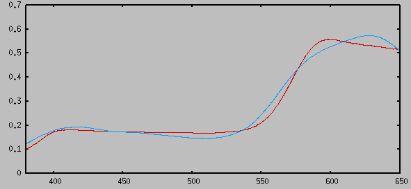
A generated reflectance spectrum made by DCamProf (blue) together with a measured spectrum from a real Munsell color patch (red). Both lead to the same XYZ coordinate when integrated with the observer's CMFs. That is this shows one example of two different spectra that produces the identical vision color.
The DCamProf spectral generator strives for smooth spectra, and its result is thus a little bit more rounded than the Munsell patch in this example.
Importing raw text data
Spectral data is often delivered in text files with the numbers just straight up listed in rows, without any header to describe the layout. Much of the data in the spectral databases linked here is in such simple text formats.
The separate command txt2ti3 (not to be confused with
Argyll's command with the same name) can be used to convert those raw
text files into .ti3 that make-target can read.
The flags should be self-explanatory so just run dcamprof
without parameters to get the information.
Example: import text spectral data (here from Lippmann2000 found in the spectral databases section) and form a target where cc24 fills out where the imported data doesn't have patches:
  dcamprof txt2ti3 -a "caucasian" -s 1 -f 400,700,2 \
    Reflect_AllCaucasian_400_700_2nm.txt caucasian.ti3
  dcamprof make-target -p caucasian.ti3 -p cc24 output.ti3
Reflectance vs emissive spectra
The default type of spectrum in a target is a reflectance spectrum, that is how much of the light that is reflected at each wavelength. Most spectral data is of this type. Reflectance spectra is first multiplied with the illuminant to form emissive spectra which is then integrated with the observer.
It's also possible to specify emissive spectra, that is light sources or reflective objects with an illuminant reflected off them. If you want to define a transmissive object such as a backlit leaf, you specify it as an emissive spectra, like a filtered light source.
In the .ti3 file the column SAMPLE_TYPE
says R for reflective spectra and E for
emissive. This is a DCamProf extension and is thus ignored by Argyll.
Observers
The observer is a mathematical model of the eye, defining its spectral sensitivity functions, or color matching functions (CMFs). It's not intended to exactly match the eye's cone response, but to provide "equal" results. The observer's CMFs have been mathematically transformed to work better in real applications.
When you integrate these CMFs with a spectrum you get the corresponding CIE XYZ tristimulus value. That is the observer is key element in modeling what colors we see.
As there's no method to actually measure the signals the eye sends to the brain the CMFs are derived from results of color matching experiments. The precision is thus dependent on the color matching skills of the people involved in the experiments.
The original observer was published as early as 1931, and it's still the number one standard observer. This is not because it's the most exact one, but because the CIE standard organization will not accept new standards unless significant improvement is made. Some minor improvements have been made over the years, but the original 1931 standard observer holds up well enough.
There are 2 and 10 degree variants of observers. The degree value refers to how large area of the eye the tested color patch covers. With the more narrow 2 degree angle the eye is slightly better at color separation, but the 10 degree generally matches real situations better. The 1931 is a 2 degree observer (1931_2), and the first standardized 10 degree observer was published in 1964.
DCamProf contains a number of observers, you can see a list when running the command without parameters. I'd like to use the 2006 observer as the default one as it's more accurate than the original 1931, and I'd also rather use the 10 degree observer as I think it matches real situations better than the 2 degree. However, as most color management software expects a 1931_2 observer and all the common color spaces sRGB, AdobeRGB, Prophoto are defined with a 1931_2 observer I've chosen that as the default. Only experiment with changing observer when you have full spectral information though, as changing observers will change XYZ values slightly so you can't have a reference file with XYZ values for a different observer for example.
If you change observer note that evaluation of profile-making results must be made with the same observer otherwise you will get larger Delta E than you should.
To get desired results with a different observer one needs at some point transform to colors for the 1931_2 observer as both DCP and ICC requires that the profile provides colors relative to that. Currently this transform model is very simplistic in DCamProf so the results will probably not be as good as they could be. Therefore consider the observer choice as highly experimental and for any production work you should stay with the default.
Examples
Re-generate XYZ reference values with a new illuminant (D65) and
observer (using the default 1931_2) for an Argyll-generated .ti3 file:
dcamprof make-target -I D65 -p argyll.ti3 output.ti3
Generate target files from scratch using camera SSF and built-in database:
  dcamprof make-target -c 5dmk2-ssf.json -i StdA -I D50 -p cc24 output.ti3
  dcamprof make-target -c 5dmk2-ssf.json -i StdA -I D50 -p cc24 \
    -p munsell output.ti3
Use the spectral generator to make targets from scratch:
  dcamprof make-target -c 5dmk2-ssf.json -i 7500K -I D50 -g 0.01 \
    -p pointer-grid output.ti3
  dcamprof make-target -c 5dmk2-ssf.json -i D65 -I D50 -p pointer \
    -p srgb-grid output.ti3
Generate a border around the Pointer's gamut and use the reserved word
illuminant to get the spectrum of the illuminant (D65 here) into the
patch set, which is necessary as with only the border there would be
no white patch:
  dcamprof make-target -c 5dmk2-ssf.json -i D65 -I D50 -p pointer \
    -p illuminant output.ti3
...and then we do the same thing by using the reserved word white to
get a perfect white reflective spectrum, which is better as
the reflective white will still work if we later change the
illuminant:
  dcamprof make-target -c 5dmk2-ssf.json -i D65 -I D50 -p pointer \
    -p white output.ti3
Re-generate both RGB and XYZ values from a previously created file which contains spectral information, use D65 for the RGB values and D50 for the XYZ values:
dcamprof make-target -c 5dmk2-ssf.json -i D65 -I D50 -p input.ti3 output.ti3
Assemble a target from imported spectra and built-in database:
  dcamprof make-target -p input1.txt -a "class1" -p input2.txt -a "class2" \
    -p cc24 output.ti3
Note that in this last case there is no SSF provided and while the input text files might have RGB values, no RGB values can be generated for the built-in cc24, and the output will thus contain dummy values (zeroes) for the RGB triplets. This means that to be used when making a profile you need to run it through again to re-generate RGB values with provided camera SSFs. For convenience the make-profile and test-profile commands support re-generation directly, so you usually don't need to re-generate reference values separately with the make-target command.
If you are using Argyll source files it's preferred that you include spectra throughout the workflow so XYZ reference will be re-generated with the observer chosen in DCamProf. If the XYZ reference values comes without spectra from a source you cannot control, it's important to know which illuminant (and observer, which almost always is 1931_2) that was used so you can later inform make-profile of that.
make-profile
  dcamprof make-profile [flags] <input-target.ti3> \
    <output-profile.json | .icc | .dcp >
Make a camera profile based on an Argyll .ti3 target file, either
generated by Argyll scanin from a raw test target photo, or by
DCamProf's make-target command. The target file contains test patches
with raw RGB values from the camera coupled with reference CIE XYZ
coordinates of the patches, and possibly also the spectral reflectance
of each patch.
The output is written in DCamProf's own native format, which can be converted later on, or if you are satisfied with default conversion flags you can directly write a DNG or ICC profile.
Overview of flags:
-n <camera name>, optional camera name. If you write DCP output directly it's important to set it.-w,-W,-v,-V, matrix optimization control parameters, documented in a separate matrix optimization section below.-l, specify LUT relaxation error ranges, documented in a separate LUT optimization section below.-a <target-adjustment.json>, apply target adjustment configuration, can be used for subjective adjustments but is mainly intended as a powerful way to control the matrix and LUT optimizers.-y <Y | X,Y,Z>smallest allowed Y (or X,Y,Z) row value in forward matrix optimization (default: −0.2 on Y only). This is typically used to avoid "unstable" matrices with large negative factors on some cameras, often blue Y. The default value limits such cameras, but also causes them to render blue a bit too light. See the section on deep blue handling for details.-k <LUT compress factor>, decides over how long range the out-of-gamut linear matrix values should be compressed at the raw level before being handled by the LUT. If set to 0 no compression will take place. The value represents the uncompressed range compared to the gamut limit (which is the intersection between the locus and ProPhoto RGB). If it's 0.7 it means that 70% of the range is uncompressed and in the remaining 30% the full range up to raw clipping is compressed to fit within DCamProf's maximum gamut. The default value is 0.7, and there's normally no reason to change it.-d <distance>, minimum u'v' chromaticity distance between patches when optimizing the LUT, default 0.02. Close patches will be grouped together and an average correction is made.-g <target-layout.json>provide target layout for glare matching and/or flatfield correction.-o, observer, default 1931_2. If the target's XYZ values are not re-generated (that is the target lacks spectra) this must match the observer used when the XYZ values was originally generated. If not known the best guess is generally 1931_2, that is the default.-c <ssf.json>, the camera's spectral sensitivity functions, only needed if you want to regenerate camera raw RGB values from spectral information in the target file.-i <calibration illuminant>, this is the illuminant the target was shot under, that is the illuminant the target's RGB values was generated for. Can be specified as an exif light-source name or number, xy coordinate, XYZ coordinate, a spectrum.json file or an Argyll SPECT file (produced by Argyll'sillumread). To allow any target value re-generation from spectra it must be a source with known spectrum. If camera SSF is provided (-c) RGB values will be re-generated.-I <target XYZ reference values illuminant>, can be specified in the same way as the calibration illuminant (-i). If spectral information is provided in the target the XYZ values will be re-generated according to chosen illuminant (and observer) when possible, and then this parameter is thus ignored. If there is no spectral information it's however important that the illuminant and observer matches what was used for the target.-C, don't model color inconstancy, that is use relighting instead of a chromatic adaptation transform.-Srender spectra if the target lacks it.-B, don't re-balance the target RGB values so the most neutral patch becomes 100% neutral (R=G=B). Per default the target D50 XYZ values used for color corrections will be remapped slightly such that the whitest patch in the target equals 100% neutral (in reality it usually differs 1 – 2 DE). This means that the ideal white balance for the profile will be the same as picking the whitest patch which is what most will expect. By enabling this flag there will be no re-balancing and instead the ideal white will be the true white, that is typically 1 – 2 DE different from the white patch. This is more of mathematical interest than having a real visible effect.-b <patch name or index>, manually point out the most neutral patch in the target. Per default DCamProf will search and find the most neutral among the lightest patches in the target, in some cases it may not be the lightest white but maybe a neutral gray below. If you want to make sure it picks a specific patch you can target it with this parameter.-x <exclude.txt>, text file with sample ID to exclude from the target, one ID per line, or Class and ID. The purpose of this file is to make it simple to remove problematic patches and re-generate the profile to evaluate changes.-p,-f,-e,-m, pre-generated matrices if you want to skip the matrix finder steps.-s, run an alternate (much) slower matrix optimization algorithm which can find a little better result. This is extremely slow and mainly intended for a last resort fallback if it seems like main matrix optimizer fails. It should thus normally not be used.-t <linear | none | acr | custom.json>, embed a tone-curve in the output DCP or ICC, and apply the default tone reproduction operator. Will be ignored if the output is the native format.-L, skip the LUT in the informational report. A LUT is always generated anyway, but if you intend to make a matrix profile in the end it can be useful to show the DE report on the matrix only while you do repeated runs tuning weights.-r <dir>, directory to save informational reports and plots.
Illuminants
It's important that you get illuminants right in order to generate a
correct profile. The .ti3 file format doesn't contain information on
which illuminant that was used for the camera raw RGB or XYZ
values. This means that you must keep track of that yourself and
provide the information to DCamProf via the -i and -I parameters.
There are a few possible scenarios:
- The target file has no spectral information, the camera RGB values were created for the desired calibration illuminant, and the XYZ reference values for some other illuminant. Re-generation is not possible.
- The target file has spectral information, DCamProf knows the spectrum of the calibration illuminant, the XYZ values in the files don't matter as DCamProf will re-generate from spectra. The RGB values must still match the calibration illuminant.
- The target file has spectral information, DCamProf has illuminant spectrum and you provide the camera's SSFs. Both RGB and XYZ values will be re-generated from spectra.
For optimal results you want to avoid the first case. That is provide
a target with spectral information, and a calibration illuminant with
known spectrum. Then all XYZ values will be re-generated from
spectra. If the target lacks spectra you can choose to simulate
them by enabling the -S flag. It cannot exactly recreate
the original unknown spectra of course, but if DCamProf has to perform
a relighting transform the results
will generally be more accurate than if not using simulated spectra.
In the most flexible case you have the camera's SSFs too. In this case also the RGB values are regenerated for the calibration illuminant you choose.
If you lack camera SSFs the RGB values from the file will be used
directly. This is the case when the file comes from
Argyll's scanin after processing your converted raw shot
of a physical test target. It will by nature contain the RGB values for the light that
illuminated the test target at the time of shooting. In this case
it depends on use case if it's important that the calibration
illuminant you specify matches the real one or not, as follows:
- If you intend to make a DNG profile and you want it to be good
at estimating the light temperature, it's important to match the
calibration illuminant. For a single illuminant DNG profile the
light temperature estimate is only informational, for a
dual-illuminant it controls forward matrix mixing and has therefore
more direct control on color correction result. You can read more
about this in the white balance
section.
- Note that for dual-illuminant DNG profiles the calibration illuminant must match a known EXIF lightsource.
- If you intend to model color appearance with CAT (enabled per default), it's important to match the calibration illuminant so the CAT gets the appropriate starting point when converting to the profile connection space which is D50.
- If you disable CAT (
-C), that is enable 100% perfect color constancy, the calibration illuminant does not affect the result, except for the DNG aspects covered in the first bullet. That is in this case it's purely informational.
DCamProf will need XYZ values for both the calibration illuminant and
the "profile connection space" which always is D50 (same for ICC and
DCP). A target file only contains XYZ values for one illuminant, and
thus the other or both must be calculated. If there is no spectral
information the Bradford CAT will be used, which does not provide as
precise results as when calculating from spectra. With the -S
flag you can enable rendering of virtual spectra which often gives a
bit better result than using the Bradford CAT.
If you have spectra the XYZ values will be generated for the
calibration illuminant first, and then converted via CAT02 to the
profile connection space D50, and in that case it's of course
important that the calibration illuminant is reasonably truthful. The
purpose of using CAT in this case is to simulate the minor color
appearance differences that occur due to the illuminant. You can
disable this behavior with the -C flag.
In any case if you shoot the target in for example outdoor daylight
you don't need to worry if you don't really know the exact
temperature. Guess one of D50 (midday sunny) or D65 (midday
overcast). If you have a spectrometer you can bring a laptop and use
Argyll's spotread to read the spectrum of the light and find
out what the correlated color temperature is so you get help to choose
the closest one. You can actually feed the actual measured spectrum to
DCamProf as well, which makes a difference if CAT is enabled, and will
make the color matrix as accurate as possible.
Here's the Argyll command for reading the illuminant
spectrum: spotread -H -T -a -s
(If you run spotread with -S, capital S, you
get a spectral plot for each measurement which can be
interesting. It's a bit user-unfriendly though, the program may seem
to lock up. You need to activate the plot window and press space to
get back to the program.)
If you lack reflectance spectra in the target file the specified XYZ illuminant must match the ones used in the target. The values could for example originate from a target manufacturer reference file, and is then often relative to D50 or D65. Make sure to look it up so you can provide the correct one. Unlike the calibration illuminant it's very important that it's exactly right.
If you have measured the XYZ reference values yourself using a spectrometer you should have spectra in the target file. If not they have probably disappeared along the way, look over the workflow and make sure it isn't lost.
Color matrix, forward matrix and LUT matrix
You may have noted that I have adopted the DNG profile names of matrices also for the native DCamProf format. This is simply because the names are familiar. It doesn't lock the native format to DNG profiles.
The forward matrix which operates in D50 XYZ space using D50 as the reference illuminant is not unique to DNG profiles, it's used for ICC profiles too. A matrix-only ICC profile can be said to contain a forward matrix. As the conversion from the calibration illuminant to D50 is needed by both profile standards DCamProf has adopted the forward matrix.
The color matrix is however DNG-specific, it's used for estimating the temperature and tint of the scene illuminant based on a white balance setting. It won't be used when generating an ICC profile.
Looking at DCRaw internals we find the color matrix again though ("cam_xyz" in DCRaw-speak), it's using a D65 color matrix per camera to render its default colors. So you can use DCamProf to contribute color matrices to DCRaw or other software that use DCRaw-style matrices.
There's also an additional matrix called "LUT Matrix". It's DNG-specific and corresponds to the best (=least bad) forward matrix that fits within the ProPhotoRGB chromaticities. This leads to a matrix with very low saturation and overall light and dull colors, but with reasonably accurate hues. It's used when generating a DNG profile with a LUT, where it replaces the forward matrix. The LUT is used to stretch colors back into appropriate positions. The reason for this is purely format-technical: while DCamProf's native format implies gamut compression of negative values from the matrix output there is no such thing in the DNG format which just clips them. By using this special matrix premature clipping is thus avoided. This is not required by ICC (Lab) LUT profiles as there is no pre-matrixing in that case.
Controlling color
For normal casual use you will let DCamProf render the profile without any added instructions, and it will then make a profile which will present the colors as accurately as possible, with suitable tradeoffs concerning smoothness. However, for advanced use you may want to control the result in more detail. This can be done in different stages in the profile making process.
The profile has a colorimetric base, which consists of a linear matrix with non-linear LUT adjustments on top. The purpose of this base is to accurately match colors, while not hurting gradients (that is not having too sharp bends in the LUT). If a tone curve is later applied then a tone reproduction operator modulates colors to compensate contrast-related psychovisual effects, and on top of that you can apply subjective "look operators". That is we have a neutral colorimetric base without any curve or subjectivity, and (optionally) on top of that a tone reproduction operator and subjective adjustments.
In theory the colorimetric base should never need any manual adjustments, as it should be close enough to being 100% accurate. That is any adjustments would be related to subjectivity and thus most suitably applied as look operators later on. In practice this is also most often the case, but color science is not an exact science and there are many sources for errors so you still may want to tune the colorimetric base in some situations. In some cases you may also want the colorimetric base to have some subjective adjustments, for example if you make a matrix-only profile and still want a subjective look, or lighten deep blues to make the profile more robust.
Here's a list of how you can control the colors and in what situations the various methods are suitable:
- Modify reference values in test target reference file.
- Modifying the reference values will of course cause DCamProf to match those new values. It's however recommended to strive for having as correct as possible values in that file, and use a target adjustment configuration on top instead, which is also easier to work with.
- Provide a target
adjustment configuration file.
- If you don't agree with the reference colors, you can change them using a target adjustment file. Normally this should only be done if your eyes think the reference color is not accurate. If you want to make a subjective adjustment (that is change to something that is not accurate, but more pleasing) it's normally better suited for a look operator later in the process. To use look operators you need to apply the neutral tone reproduction operator though which requires a LUT, so if you make a matrix-only profile you need to use target adjustment also for subjective adjustments.
- Even for LUT profiles there are exceptions when you may want to make subjective adjustments already in this stage. A typical example is to lighten deep blue to make the profile more stable when handling extreme colors. Another reason is that it's generally much easier to make strong subjective adjustments here than in a look operator; look operators are better suited for small subtle adjustments.
- Matrix optimization.
- As a LUT is normally applied on top of the matrix to correct residual errors it's generally not important to manually control matrix optimization. However if you make a matrix-only profile you may want to have more precise control of the tradeoffs.
- Per default DCamProf treats the full colorspace as equal and tries to minimize the errors all over. A modern camera can usually match colors quite well with just a matrix, but there's still often up to 3-4 DE on some colors on a typical target. You can manually control the tradeoffs and for example let colors you consider more important become more accurate at the cost of other less important colors.
- If you're a perfectionist you may even for a LUT profile still want to control the matrix. The reason is that the LUT tries to be as close to the matrix as possible, as it means ideal gradients, so the closer the matrix is to the desired end result the better.
- Refining the optimizer results is about placing the unavoidable matching errors where it hurts the least; if you really want to change what colors the optimizer strives for you should alter the reference colors using a target adjustment configuration.
- LUT optimization.
- LUT optimization is a tradeoff between accuracy and smoothness.
- Per default DCamProf prioritizes smoothness (avoid sharp bends in the LUT) and tries to stay quite close to the underlying matrix-only color, and doesn't even correct lightness at all. This can be manually controlled though, and you can if desired match all patches in full, but that will most definitely hurt smoothness.
- It's quite risky to manually control LUT optimization as it may be difficult to first notice that smoothness has been hurt. The various plots DCamProf can provide is useful to analyze the result.
- The typical use case for manual control of the LUT is when you have some key colors that need very good matching. If it's only one color (or possibly two) you could consider matching them already with the matrix though.
- Tone curve, and tone reproduction operator.
- The choice of tone curve and tone reproduction operator has a distinctive effect on the look, as described in the section about tone curves.
- Gamut compression, will affect the appearance of high saturation colors.
- Look operators.
- A specific configuration format for subjective adjustments placed on top of the tone reproduction operator.
- Made specifically for designing a subjective look.
Unless you use the ICC or DNG profile output presets, the make-profile command will make a DCamProf native format profile and that only contains the colorimetric base, that is the matrix and LUT, but no tone curve, gamut compression or look operators which are all added in the final step when you make an ICC or a DNG profile.
Patch classes
To control the matrix and LUT optimizers you need to be able to
address the patches. If you have a large target, perhaps hundreds of
patches, it may not be feasible to address them one by one. For this
case the target file can be split into "classes" (=groups of patches),
specified through a SAMPLE_CLASS column in the target
file. The idea is that you can have class names such as "skin",
"forest_green", "textiles" etc and then for example assign greater
importance to skin-tones.
Class names in the target file is a DCamProf concept and is not
available in Argyll-generated files. By running an Argyll file
through dcamprof make-target -p argyll.ti3 -a name
out.ti3 you can add a class column, and then edit the text file
manually and change names to split into more classes if you like. That
way you can split even a 24 patch color checker into several
classes. It's more often used to separate different spectral sources
when making composite targets though.
Matrix optimization
For most uses you can let matrix optimization be fully automatic. If you still do want to control it it's possible using weighting and refinement parameters.
The matrix is the linear base which the LUT applies its non-linear corrections to. If the matrix is close to the ideal, the LUT needs to stretch less which makes it easier to manage. Relaxing the LUT makes gradients smoother and the result closer to the matrix. This means that it's a good idea to have the matrix close to your desired end result.
A matrix is by nature perfectly linear and thus have no issues with gradients (smoothness). It can however be more or less precise, and be more or less robust when it comes to extreme saturation colors.
There are a number of ways to control the matrix optimizer:
- Assign weight to patch classes or individual patches (parameter
-w). - Limit the XYZ negative range (parameter
-y). - Exclude patches from the target (parameter
-x). - Provide refinement error ranges per patch class or individual
patches (parameter
-v).
-w parameter, and
defines how important each patch should be. If you do provide weights
you should cover the whole target. If you have 24 patches and all
patches get weight 1.0 except one patch that gets 2.0, the matrix
optimizer "sees" a target with 23 × 1.0 + 1 × 2.0 patches,
so that patch with twice the weight will be considered a bit more
important.
Using patch weighting is rather crude, which is a side-effect of the mathematical optimizing process itself which is difficult to steer in specific directions. It's generally not that effective for fine weighting, such as differing between several normal range colors like preferring skin-tone precision over forest greens; the matrix optimizer is likely to find some similar "best" anyway. It can be more effective if you for example group high saturation colors (from a glossy target) in one class and normal saturation colors in another. For example you may want the matrix to be precise on normal range colors and worry less about high saturation colors and then you could set the weight to 0 for your glossy class (same as excluding them).
DCamProf makes a pre-weighting per default (the user weighting is
added on top), this is to handle the situation when you combine
several patch sets with different density. Some patch sets may have
lots of patches concentrated around some specific color, and another
may have few patches widely separated. This is common when using
spectral databases. To not cause the dense sets to totally dominate,
there's a pre-weighting based on Delta E distances that normalizes all
patches. This is generally a good thing, but if you really want that
one patch should equal one weighting unit you can disable this
normalization by adding the -W flag. This normalization
only affects the matrix optimizer. There is little reason to disable
it.
If you have a simple target like the CC24, you will probably not do any matrix weight adjustments at all, as it doesn't really change much in practice.
Next up, you can limit negative components in the matrix which
generally has a much stronger effect than patch weighting. As
discussed in the extreme colors section
a matrix which matches normal colors well may get strong negative
components and cause for example deep blues clip to flat blue or even
black. By limiting the negative components this is avoided, and as a
side effect the affected color range will be lightened (which often is
a desired subjective effect in any case). Although the LUT will
counter-act and correct to get the same result regardless of the
matrix, when you relax the LUT you will get closer to the matrix
result. This limiting value is set with the -y
parameter. If you want to use it a typical start value could be
-0.1. Note that the matrix optimizer uses this as a guide, the actual
result can be slightly different (that is it may break the -0.1 limit
anyway). Read the section on custom
deep blue handling to get some further information on how this
can be used.
The default value of -y is -0.2 and will thus limit the
matrix of some cameras. This can have a quite strong effect, nearly
always showing as a lighter blue (can be seen on the C01 deep blue
patch on a CC24). If you want to start off with an unbounded matrix,
which can be a good idea when you experiment with weighting, provide a
large negative like -y -5 to make sure the matrix won't be
limited. The default value is there for a reason though,
cameras that are limited by this value is likely to perform in
unstable ways in the deep blue range if it's rendered "on the mark".
If the matrix optimizer would for example make your red
colorchecker patch a little bit too magenta (probably due to a
trade-off with other patches), you could in theory create a separate
class for that red patch and assign it a much higher weight. This is
however not likely to work well. If you want to achieve precise
hue-changing results of the matrix optimizer you should use
the target adjustment
configuration and simply reduce the magenta component of the reference
value, possibly exaggerate to get the desired effect. Adjusting the
target is normally not needed, but it's there for those that need
precise control of the matrix result. You may want to use target
adjustment only for the matrix, but not for the LUT optimizer. In that
case you need to design the matrix first, and the LUT later. You do
this by ignoring the LUT result first (use -L parameter in
make-profile and make-dcp/make-icc commands), and when satisfied with
the matrix you store it in a separate file and provide that to a new
make-profile run with the -f, -m and -e
parameters.
Another powerful way to affect matrix optimization is simply to remove
patches, equivalent to assigning 0 weight to them. While you could cut
it from the target file itself, it's generally easier and more
flexible to use the -x parameters and provide a list of
patches to exclude. Again this affects also the LUT optimizer, so if
you only do this for matrix control you need to do separate
runs. Removing patches usually has a quite strong effect on the
result, but is hard to predict. I only recommend to remove patches if
you have those that seem problematic (often caused by a bad
measurement).
The matrix optimizer is locked to preserve the white point, that is it will always match the white point perfectly. This is required by DNG profiles by definition, and is in general a good idea (as the eye is very sensitive to neutrals) so it's not possible to turn off this aspect of optimization.
During optimization DCamProf will try to
match all patches and minimize all errors (taking weighting etc into
account), and then perform a final refinement step when the white
point is preserved. However it's also possible to provide an own
refinement step added on top (and then an additional white point
preservation step is run at the end, as the white point must always
match). This refinement is provided using the -v
parameter, and is applied both on the ColorMatrix and the
ForwardMatrix (if you only want it applied to the forward matrix,
provide the -V parameter).
You can specify several refinements on the same command line, by
repeating -v with more patches or patch classes. A
refinement is an acceptable DE error range, specified in all three
dimensions (lightness, chrome, hue), for example like this:
-v A02 -0.5,1,-3,2,-0.3,1.5
The above addresses the patch "A02" and says that the patch must be no darker than -0.5 DE L than the reference value, no lighter than +1 DE L, no more desaturated than -3 DE C, no more oversaturated than +2 DE C, and hue must not be more than 0.3 DE h off counter clockwise or 1.5 DE h clockwise. You can specify hue in one dimension if you like, that is provide just 5 numbers instead of 6. If the error is already within the specified ranges, no refinement will take place.
As the matrix is linear all patches are interconnected, this means
that if you improve one patch, the patch for some other patch(es) will
get worse, so this is very much a trial-and-error process. Activate
the -L and dump report files -r look at the
patch matching images and repeat until you get the desired result.
Some refinement combinations will be impossible to meet with a matrix, and then the make-profile run will fail with an error message.
Refinements are powerful but can be a bit cumbersome to work with. It's easiest to work with on small targets, like a CC24, where it's easier to get an overview of how much a refinement hurts precision of other colors. If you work with refinements specifying one to three of them is generally feasible, more than that it's often hard to get to a solvable matrix. For example you could use refinements to make a great match on skin tone, avoid deep blues getting darker than they should, and make sure that reds are pulled towards orange rather than purple, and blues to cyans rather than purple. This refinement could look like this on a CC24:
-v A02 0 -v C01 0,2,-1,1,-2,0 -v C03 -3,3,-3,3,0,3
In the above example it's demonstrated the special case when only a single DE number is used, in this case 0, which is an alternative to specify each axis range separately. To actually work with this your command like could look like this:
First a base run to see how the unrefined matrix looks:
dcamprof make-profile -L -r dump cc24.ti3 dummy.jsonLook for
dump/fm-patch-errors.tif to see the
ForwardMatrix matching, save it to a separate name and use as
reference. Then using trial-and-error provide refinements over and
over again, maybe ending up like this:
dcamprof make-profile -L -V \
  -v A02 0 -v C01 0,2,-1,1,-2,0 -v C03 -3,3,-3,3,0,3 \
  -r dump cc24.ti3 profile.json
For each trial run compare with the original result to see where the matching results got worse and where it got better. In this example the
-V flag is activated which means that the custom
refinements are only made on the ForwardMatrix. As the ColorMatrix is
only used for white balance calculations in DNG profiles and not color
rendering it makes sense. However if you're making an old-style DNG
profile without ForwardMatrix or you want to export the ColorMatrix to
some other context you may want to refine that too, and then you
should not include the -V flag. The LUT Matrix cannot be
targeted for custom refinements; as it's only a format technical
matrix it doesn't make sense to do so anyway.
LUT optimization
A LUT can always stretch, compress and bend to match the target patches exactly, but that can result in sharp and even inverted bends causing ugly gradient transitions (typically most visible in photos with strong out-of-focus blur backgrounds when one color transitions into another). In this case it's better to relax the fitting, and the LUT optimizer will automatically relax in the best way based on the provided acceptable Delta E ranges (in CIEDE2000).
The LUT optimizer will per default add automatic DE ranges which will
make a smooth LUT, so for casual use it's not necessary to control
it. Advanced users may want to do so though, and then you use
the -l parameter, in the simplest case you just specify
one number, like -l 2. This instructs the LUT optimizer
that an error of 2 Delta E is acceptable, and relaxes the stretching
towards the linear matrix either until reaching the matrix or the
error reaches 2 Delta E. If you set a very large number the LUT will
be able to relax so much it becomes identical to the matrix result.
You can also specify this per patch or patch
class, in this case you specify the name first and then the Delta
E range(s), for example like this: -l skintone 1 -l glossy
4, assuming we have the class names skintone and glossy. If
you do such naming you should have names for all patches so you can
specify range for them all. Those that are not named will be kept at
their automatic values (stretch to "suitable" accuracy).
Instead of just providing one number you can specify the range exactly in all three dimensions in order lightness, chroma (saturation) and hue. For example:
-l -1,4,-3,2,1.5
This configuration specifies that in lightness patches may be no more than 1 DE darker, but up to 4 DE lighter is okay; in chroma we say up to 3 DE desaturation is fine, but only 2 DE over-saturation, and hue range is specified only with one number in the example and this is set to 1.5 DE (it can be specified with two numbers to if direction is important). Lightness errors are generally the least disturbing, indeed easy to detect when doing A/B swapping tests but it doesn't look "wrong" if you just look at one picture isolated. However it can often be a good idea to not let patches become too dark as it will hurt tonal visibility, thus specifying a tighter range in the dark direction is a common strategy.
Most modern cameras have widely overlapping filters and are therefore naturally desaturated on the raw level. Pushing for more saturation is thus likely pushing the profile into more stretching. Over-saturated patches is also arguably more disturbing than under-saturated. Thus a chroma range with larger negative DE than positive is also a common strategy.
Generally we want hues to be as exact as possible, but if we don't provide any relaxation at all it will become hard for the LUT to relax also in the chroma direction, so setting some non-zero value is recommended. If you like you can specify a range also on the hue. Hue is ordered magenta-red-yellow-green-cyan-blue, so if you for example want a blue color to rather become cyan than magenta you could specify the hue range as -2,0. For many cameras it may be a good idea to try to not fall into the line of purples unnecessarily as it can make a more unstable profile when handling high saturation colors.
You can disable correction all-together on an axis, simply by setting very large DE values (say 100). Disabling the lightness axis is a common strategy (which is employed in the default automatic mode) as lightness suffers more from measurement errors (glare) and is more likely to disturb gradients than chroma and hue corrections.
Note that LUT relaxation is somewhat approximate, which means that if
you specify a relax of 2 DE you may not end up exactly at 2. Also note
that as the LUT is 2.5D some patches may be grouped together and thus
cannot be corrected individually, so even if you provide -l
0 some patches will not reach DE 0.
White balance
You can control white balance settings with the -b and -B
parameters. Per default DCamProf will make a profile which expects the
white balance to be set by color picking the most neutral light
patch. In some cases the target "white" is actually considerably less
neutral than a darker neutral gray patch, if so that will be used
instead. If you are going to use the target as white balance setter
for a scene it's safest to specify a specific patch as reference, you
do that with -b.
The most accurate correction is however had if you let DCamProf
optimize towards a virtual 100% neutral patch, this will typically
place the ideal white balance a little bit off the target's
white. As it's only about 1-2 DE it's really only of mathematical
interest though, it shouldn't make a visible difference in any normal
circumstance. If you want to do this you enable the -B flag.
Note that this only affects the forward matrix (which is used for the color corrections), the values used for color matrix calculation will not be re-balanced as it doesn't make sense; it's not used for color correction but only for estimating the light's temperature and tint and thus re-balancing its data would only reduce its precision.
If you're working with SSFs and virtual targets you probably already have a perfect white in the target and then this setting will make no difference.
Target adjustment
While you can affect matrix optimization a little bit with weighting,
if you really want to adjust how it matches a color (typically hue),
changing the XYZ reference values is the easiest and most powerful
way to do it. You could change directly in the target .ti3
file but if you work with spectra (like you hopefully do) it's not
feasible.
Therefore DCamProf provides the option to provide a target adjustment configuration file in JSON format, a documented example is provided in the data-examples directory. You can make global adjustments without pointing out specific patches, but those will only take effect if there is an actual patch matching the changed area. If you have relatively few patches (like for a CC24) the easiest way is to target individual patches.
In earlier versions of DCamProf the intention was to control the matrix optimizer with DE range specifications, like the LUT relaxation is controlled. However, due to the specifics of matrix optimization that method becomes much too unreliable and unpredictable. Adjusting the reference values works a lot better for this task.
So while you can make subjective adjustments this way, you could also do this to compensate some error in the process (maybe bad reference values), or if you just want to shift which colors the matrix optimizer matches best. If you're making a matrix-only profile in the end you can make strong and "wrong" adjustments as long as the matrix optimizer result suits you.
If you're into the subtle parts of custom looks, you should be looking to use look operators instead which is applied when you generate the DCP or ICC profile.
Deep blue handling
As discussed in the section about extreme color handling deep high saturation blues can be a problem, especially with certain cameras. For normal colors this is not a problem, but if you often shoot nightscapes or nightlife where artificial emissive light sources can trigger strong blue response you may experience a problem with a normally designed profile.
You can diagnose your camera's blue sensitivity in the resulting
ForwardMatrix: if the middle row value of the third column (raw blue
multiplier for CIE Y output) is more negative than say -0.15 your camera is
likely to have some issues in this range. To diagnose you need to make
sure the Y is not limited when making the profile though, by setting
the -y parameter to a large negative value. It's set to -0.2
per default which means that problematic cameras will render blues too
light, but will yield more robust profiles (the default is there to help
casual users).
There is another reason to handle blues in a custom way: the eye is not very sensitive in the deep blue range, so it's harder to see tonal variations in that range. Therefore many commercial general-purpose profiles render deep blues much lighter than they are experienced in real life, making tonal variations more visible.
Normally these subjective "look" adjustments are made using look operators, which indeed from a design perspective is cleaner: that is you develop a a profile which is as accurate as possible in a colorimetric sense, and on top of that you make subjective adjustments. However from a practical processing perspective it's sometimes better to introduce some subjective adjustments already at the colorimetric stage. Limiting the blue range and render it lighter is one such case, and the reason is to minimize potential clipping and gamut compression in the base profile. If the colorimetric base has strong compression in the blue range it's hard to restore using a look operator. That is by lightening blue in the colorimetric profile we have a better chance to maintain optimal tonality in the range.
There are two ways to control the blues. 1) you can limit the range in
the matrix, forcing the optimizer to subtract less blue than it does
when optimizing freely (use the -y parameter, for
example -y -0.1). And 2) you can provide
a target adjustment
configuration file and lighten blue patches there. For the
classic CC24 the C01 patch gives good control of deep blue.
The eye is more sensitive to greens and reds and camera matching is less problematic there, so you generally don't need to make this type of handling for other colors.
Here's a real-world example for a Sony NEX6 which is problematic in the blue range:
dcamprof make-profile -y -0.15 -a adjust.json cc24.ti3 profile.json
Here we have a target adjustment file too (adjust.json), we choose to
make the blues a bit less red as it in this case makes the matrix even
more robust:
  {
    "PatchAdjustments": [
      {
        "Name": "C01",
        "ScaleRGB": [ 0.8, 1.0, 1.0 ]
      }
    ]
  }
That is we've reduced red (0.8) of the deep blue patch (C01) in the CC24. If you're doing any hue adjustment of deep blue reducing red and/or increasing green (that is pull it away from magenta towards cyan) is often a good idea. An unstable deep blue that gets a tiny bit too much red in it quickly becomes a strong magenta, which is very different from blue. The transition to cyan is less conspicuous and in terms of look it fits better, looking like an "over-exposed blue".
Profile-making tips
Do experiment! Learn how to use a plotting tool and plot results. To get a general feel of how profiling works in practice you can play around with one of the example camera SSFs, and then use the acquired knowledge when you tune settings for your targeted camera (for which you often don't have SSFs).
What you will see is that there is no such thing as a perfect result, and the farther from the whitepoint you get tougher it will be to compensate errors. While it can be fun to try to get a profile that works all the way out to the gamut limit it will hurt performance of common colors. It's generally better to maximize performance for colors you're actually going to shoot. Pointer's gamut approximates the limit of how saturated real reflective colors can be, colors outside that need to be represented by emissive (or transmissive) light like lasers and diodes. It's generally not worthwhile trying to get a good match outside Pointer's gamut. If you have the camera's SSF you can plot and see how well the camera can actually separate colors, you will probably see that there are some issues when it comes to extremely saturated colors, and no camera profile can compensate for that.
Consider that a perfect match to a specific color checker doesn't mean that the color precision is perfect, not even for those colors. It's only perfect for the particular spectra the color checker has, somewhat compromised by various measurement errors throughout the profile making process. Therefore I suggest to always apply some LUT relaxing to smoothen profiles at least some. As true perfection cannot be had, it's better to make sure color transitions are smoothly rendered.
If you see very large errors after matrix-only correction, say 10 DE or more, the LUT may get a too tough job and be forced to make extreme stretches than can make bad gradients and an unpredictable profile. One way to test a profile for robustness is to load it in a raw converter, show a color checker with many colors, and change white balance. If some color suddenly changes must faster than the others the LUT is probably making a strong local stretch at some point. Of course you can see this by plotting as well, but the white balance test is a good and simple sanity check.
Modern cameras should get a decent match of normal colors with the matrix alone, so if you do see large errors, such as 10 DE or more, it's likely that there is some wrong with your input data, such as poor lighting of the test target, glare, bad references values or reflectance spectra.
Make sure to check what the dynamic range test shows (printed in the console output when running make-profile). Example output:
Camera G on darkest patch(es) is 9.8% lighter compared to observer Y.
  Y dynamic range is 4.78 stops, G dynamic range is 4.64 stops, difference
  0.14 stops. A small difference is normal, while a large indicates that there
  is glare.
In the above example there's only 0.14 stop difference, and up to
about 0.25 should be okay (that is very small effect on profiling
result). By using the -g parameter and providing a target
layout description you can let make-profile model the glare to
compensate. This is usually a good idea, but don't expect perfect
results for high amounts of glare.
Note that you can only trust the dynamic range test result if the target has pure black patches. If the darkest patch is colored it's a large risk that the result is misleading.
Examples
In all examples below it's assumed that the target file contains reflectance
spectra. If not you need to specify the XYZ reference values
illuminant using the -I parameter.
Example 1: basic profile making with default parameters, using calibration illuminant StdA (calibration illuminant = the light source the target was shot under):
dcamprof make-profile -i StdA target.ti3 profile.json
Example 2: assuming we have a target with CC24 and the border of
Pointer's gamut, we
make sure the matrix is more focused on matching the CC24 (weight 1)
than the Pointer border (weight 0.5). This sets up the matrix for
requiring less LUT stretch for normal colors. Then we specify the LUT
max acceptable Delta E ranges, generally accepting less darkening than
lightening, and less over-saturation than under-saturation, and
requiring better precision of CC24 than Pointer. We specifically allow
the Pointer border to be quite desaturated (-4). By providing
camera's SSF (-c) the RGB values will be re-generated for the given
illuminant (D65). Data files for plotting are saved to the "dump" directory (-r).
  dcamprof make-profile -r dump -c ssf.json -i D65 \
    -w cc24 1 -w pointer 0.5 \
    -l cc24 -0.5,1.5,-1,0.5,0.7 -l pointer -2,4,-4,1,2 \
    target.ti3 profile.json
Example 3: applying matrix optimization refinements to three patches
(-v) only to the forward matrix (-V). Data
files including patch matching report images useful for evaluating the
refinement result are saved to the "dump" directory
(-r). By using -L the printed matching
report will not include the LUT (the LUT is generated anyway though)
so we can directly see the matrix matching.
  dcamprof make-profile -r dump \
    -V -L
    -v A02 0 -v C01 0,2,-1,1,-2,0 -v C03 -3,3,-3,3,0,3
    cc24.ti3 profile.json
Example 4: make matrices using one target, and the LUT using another by running make-profile twice, first making the matrices and then the LUT:
  dcamprof make-profile -i D65 target1.ti3 m.json
  dcamprof make-profile -i D65 -m m.json -f m.json -e m.json \
    target2.ti3 profile.json
test-profile
  dcamprof test-profile [flags] [target.ti3 | test.tif]
  <profile.json|.dcp|.icc> [output.tif]
The test-profile command is used to 1) test how well a profile can match
a specific target, or 2) skipping the target it will only run
diagnostics on the profile, or 3) replacing the target with a TIFF
file it will pass that through the profile. The output.tif is
optional. If provided a test gradient or the processed input TIFF will be
stored there, otherwise in the report directory (if enabled).
It will print a text summary on the console, for deeper information
you should use the -r parameter to dump text files and plots.
As always it's preferable that the target file contains spectra so XYZ reference values can be re-generated rather than having to be converted using a chromatic adaptation transform.
Overview of flags:
-o <observer>, used if patch values are re-generated, default 1931_2.-c <ssf.json>, the camera's SSFs, used to re-generate target RGB values, or if you want to analyze the camera's color separation performance.-i <test illuminant>, the illuminant the test is run under, which per default is the same as the profile's calibration illuminant.-I <target XYZ reference values illuminant>, default is same as the test illuminant. Only required if the target lacks spectral data.-C, don't model color inconstancy, that is use relighting instead of a chromatic adaptation transform.-Srender spectra if the target lacks it.-b,-B, white balance settings, see make-profile for documentation.-w <r,g,b> | m<r,g,b>, provide camera white balance as RGB levels or RGB multipliers. Per default white balance is derived from the target, or when provided from the camera's SSFs.-L, skip LUT. If the profile has a LUT but you want to test how it performs with only matrix correction enable this flag.-P, skip DCP LookTable LUT. Only applicable to DNG profiles, and only applicable to certain tests, in colorimetric matching tests it's generally excluded anyway (if there is a HueSatMap).-T, skip adding Adobe's default tone curve to DNG profiles that lacks curve. Note that the colorimetric tests won't use the curve anyway though as it doesn't make sense.-f <file.tif | tf.json>de-linearize RGB values in target, that is run the provided transfer function backwards. This is only relevant for ICC profiles made for raw converters that apply a transfer function, such as Capture One.-r <dir>, directory to save informational reports and plots.
White balance
Per default DCamProf will calculate the optimal white balance to match the target as well as possible. This is analogous to setting white balance in your raw converter with the white balance picker on the white patch on a color checker. You can adjust this white balance behavior in the make-profile command, and if you have done that you should mirror the same settings in the test-profile command.
If you instead want to test how the profile will match colors
when the camera is set to a different white balance (such as a camera
preset) you can provide a custom white balance via the -w parameter.
It's given as a balance between red, green and blue, or as channel multipliers. To find out what multipliers a camera is using you can run exiftool with a raw file. White balance can be stored in different ways depending on raw format. In most cases it's some sort of multipliers though, and green is often repeated twice, like this:
WB RGGB Levels Daylight : 15673 8192 8192 10727
Then you simply provide -w m15673,8192,10727 to
DCamProf, note the m which specifies that we provide white
balance as multipliers rather than actual resulting balance between
the channels which is 1/m.
When DCamProf prints a white balance it will show the resulting balance
normalized to 1.0, meaning that the above example translates
to 0.52,1,0.76.
Analyzing camera color separation performance
There is a special feature embedded in the test-profile command, which is that if you provide the camera's SSF you can get an analysis of the camera's color separation performance. This is a pure "hardware" test and has thus no relation to the profile so if you are only interested in this result you can provide a dummy profile.
This feature should be considered as experimental.
To get a sane result you need a highly populated grid of patches to test with. I recommend to generate a locus grid, like this:
dcamprof make-target -c cam-ssf.json -p locus-grid -g 0.01 locus-grid.ti3
This will take quite some time, but once generated you can reuse this grid with any camera since when you provide the SSF and illuminants the RGB and XYZ values will be regenerated from spectra:
  dcamprof test-profile -r dump1 -c cam-ssf.json -i D50 locus-grid.ti3 \
    any-profile.json
To get the plot you need to provide the -r parameter, and then the
file is named ssf-csep.dat. You can plot it using
this gnuplot script:
  unset key
  set palette rgbformula 30,31,32
  set cbrange [0:300]
  plot 'gmt-locus.dat' using 1:2:4 w l lw 4 lc rgb var, \
    'ssf-csep.dat' pt 5 ps 2 lt palette, \
    'gmt-adobergb.dat' w l lc "red", \
    'gmt-pointer.dat' using 1:2:4 w l lw 2 lc rgb var
You will then see a heat-map in a u'v' chromaticity diagram, here limited to 300 max. Each tiny square shows how much the camera signal will change in 16 bits (65536 steps) for 1 Delta E unit change in chromaticity (= change in hue and saturation with constant lightness). No current camera is really 16 bit, it's used here as a fixed reference to get a number in a comfortable-to-read range. For this type of test where we look at performance in of well-exposed colors we should not worry about a camera's dynamic range and read noise, instead shot noise will be the limiting factor.
A black square means that the signal change is zero and thus the camera hardware cannot separate color at that chromaticity location and no profile can ever change that.
The test is run against the target provided and it expects a dense grid-like layout of patches. If the target is coarse the results can be misleading. The locus grid generated in this example makes reflectance spectra, so the colors tested are all related to the illuminant, and the colors are as light as the illuminant allows for that chromaticity. This means more saturated colors are naturally bit darker and thus harder to separate. However it becomes harder for the eye too. Cameras will often show good separation capability in the purple range, and that is partly because the eye is relatively poor at it. As the values are related to Delta E they will be related to the eye's capability (as modeled by the observer's color matching functions).
The diagram always shows values relative to a D50 white point. You can
test with a different illuminant using the -i parameter. You will see
the result changing, but the coordinates are always remapped to D50 in
the diagram.
Note that the generated locus grid will not go all the way to the edge of the line of purples. This is because the line of purples is actually black (as it's at the border of the eye's sensitivity) so by moving it in a bit we get saner colors. The spectral generator can still have some issues to reach all the way to the locus and line of purples so you may get some gaps.
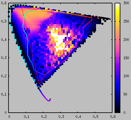
This diagram in u'v' chromaticity coordinates shows the color separation capability of a Canon EOS 5D Mark II. The locus, Pointer's gamut and AdobeRGB gamut is shown as reference. Only points that have a patch in the provided target will be plotted, so here you see some gaps at the borders where the spectral generator did not succeed making test patches (which is normal).
The unit of the heat map is how many 16 bit units (65536 steps) the camera raw signal changes if the color chromaticity changes with 1 CIEDE2000 unit. The test reflectance spectra is a generated grid related to a D50 illuminant, and is made as bright as possible for each chromaticity coordinate.
The darker heat (lower signal difference) the worse color separation, if it's zero the camera can't differ at all. For complete information of limits you need to relate to photon shot noise as well, which is out of the scope of this document. What we can see is that the camera gets problems towards the locus, mainly on the cyan side and towards the red corner. We also see it's good at purples, which is partly due to that the eye is not as good and thus it takes more distance to reach one delta E.
We can also see that the diagram is a bit "worried" and that we have a notable minima inside AdobeRGB towards the red corner on the purple side. Some odd minimas here and there and the messy look is typical, as the SSFs differs greatly from the observer's CMFs. We see a smoother behavior in the green area, this is because there all three SSFs are involved in producing the signal.
Gradient testing
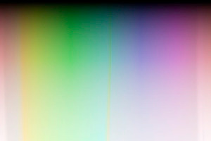
Example crop from the gradient test file showing a few poor transitions, such as the yellow vertical band in the center
If you enable -r <dump> a generated gradient TIFF file will be
dumped, first without any processing as gradient-ref.tif and then
processed through the profile including the LUT(s)
as gradient.tif. This means that the
content in gradient-ref.tif corresponds to white-balanced
raw camera data, and the output is what that becomes when processed
through the profile.
The purpose of this is to diagnose the smoothness of the profile's LUT as a complement to plotting. Note that as the gradient goes through all combinations (with some spacing) there will be some "impossible" raw values too, for example maximum blue but no red and green output. It's quite common that a profile clips or make artifacts in those areas, but this is no problem as they won't appear in real images.
This artificial gradient image is also very useful for verifying the smoothness during design of a subjective look using look operators.
The RGB primaries in the output is ProPhoto, and an ICC is embedded in
the files. Beware that poor gradients and clipping is likely to occur
due to the screen's color management, so turning it off temporarily
when analyzing the more saturated parts of the image may be
worthwhile. Use the unprocessed gradient-ref.tif for sanity
checking; if that shows banding or other artifacts it's probably due
to the color management of the display.
Custom image testing
If you provide an image instead of a target file it will be processed by the profile:
dcamprof test-profile test.tif profile.dcp output.tif
The source image must be an 8 or 16 bit ProPhotoRGB TIFF image. The
linearized data will then be interpreted as white-balanced camera raw data
and processed through the profile, and then saved to a new ProPhoto RGB
image (output.tif).
One use for this is to test a look design on some specific
subject. In that case you typically don't want to test the camera
colorimetric profile at all, but just analyze the effects of the
look. To do this use the nil-profile.json in the
data-examples directory to render an ICC or DCP:
dcamprof make-dcp -t acr -o look.json nil-profile.json test.dcp
And then you process your test image with that profile:
dcamprof test-profile test.tif test.dcp output.tif
The test image should be a normal white-balance image without a curve and with ProPhotoRGB ICC profile. You can prepare it from a real raw file, just make sure you apply a basic profile without a curve and export to a 16 bit ProPhotoRGB TIFF.
The common way to test a look is to apply a normal finished profile on a real raw file in a raw converter. An advantage of applying it to a TIFF file using test-profile instead is that you can merge several images into one to test several aspects of the look at once. You can also make artificial images, to test gradients or special hue ranges that are difficult to find in real images.
Examples
Example 1: test how well profile.dcp matches target.ti3 under illuminant StdA,
and write analysis data files to the directory dump (it's
assumed target.ti3 has spectra, if not you need to provide the -I
parameter too):
dcamprof test-profile -r dump -i StdA target.ti3 profile.dcp
Example 2: test how well the profile will match colors with a camera white balance preset (found out via exiftool for example):
dcamprof test-profile -r dump -w m15673,8192,10727 -i D65 target.ti3 profile.json
Example 3: disable the profile's LUT and see how well the matrix matches the target (note that DCPs may be designed such that the matrix is very far from correct color and the LUT is required to get close):
dcamprof test-profile -r dump -L -i D65 target.ti3 profile.dcp
Example 4: don't run any patch matching test, but only dump analysis data:
dcamprof test-profile -r dump profile.dcp
make-dcp
dcamprof make-dcp [flags] <profile.json> [profile2.json] <output.dcp>
The make-dcp command converts a profile in DCamProf's native format to Adobe's DNG Camera Profile (DCP) format, which then can be used directly in raw converters that support DNG profiles.
Overview of flags:
-n <unique camera name>, must match what raw converters are expecting, provide within quotes.-d <profile name>, the profile name tag string, used by some raw converters (like Lightroom) in the select box when choosing profile to use, so come up with a name that makes the profile easy to identify. If there are spaces in the string, provide within quotes.-c <copyright>, the copyright tag string. If there are spaces in the string, provide within quotes.-b <baseline exposure offset>, optionally set the baseline exposure offset tag.-B, don't include the DefaultBlackRender=None tag, meaning that some converters will then do automatic black level adjustment. If you're a Lightroom user you're probably used to automatic black level adjustment and may want it also for your DCamProf profile, and then you should enable this flag.-i <calibration illuminant 1>, specify a different calibration illuminant 1 than the tag found in the source profile, useful if the source has "lsOther" and you're making a dual-illuminant profile.-I <calibration illuminant 2>, specify a different calibration illuminant 2 than the tag found in the source profile, useful if the source has "lsOther" and you're making a dual -illuminant profile.-m <other.dcp>copy illuminant(s) and color matrices from the provided DCP. Do this if you want your profile to calculate white balance the exact same way as the provided profile. This is useful if you need to avoid a white balance shift.-h <hdiv,sdiv,vdiv>, hue, saturation and value divisions of LUTs (default: 90,30,30). The value divisions is only used for 3D LUTs. The 90,30,30 is more dense than usual and yields a large 3D LUT (total profile becomes about 1.5 megabytes). The reason for this default is that the 3D LUT is used by the neutral tone reproduction operator and it needs a high density to work well as it counteracts some of the look problems produced by the DCP tone curve.-v <max curve matching error>, used to automatically calculate value divisions needed for the LookTable when applying a neutral tone operator. The default should do (0.0019).-F, skip the forward matrix, will generate an old-style DNG profile without forward matrix. This is not recommended but may in some rare situations be necessary as some ancient software doesn't support forward matrices.-E, don't use the special LUT matrix as forward matrix in your LUT profile, but instead use the actual forward matrix. This can be desired if you use it in a context where the LUT can be disabled (like RawTherapee) and you need good colors even then. The drawback is that extreme value handling will be worse as the matrix clips, unless the raw converter has built in handling for that.-L, skip LUT (= matrix-only profile).-O, disable forward matrix whitepoint remapping. It's generally not a good idea to disable as it may render the profile unusable in some DCP software.-G, skip gamma-encoding of 3D LUTs. This only applies if a 3D LUT is used. Normally the value channel in the LUT is gamma encoded as it better matches the eye's lightness sensitivity and we get a better use of value divisions. It may lead to compatibility issues with older/simpler DNG software though. If using this flag, consider increasing value divisions to retain precision.-D, make the HueSatMap 3D instead of 2.5D. In general this makes a very small difference but the profile considerably larger.-H, allow hue shift discontinuity between LUT entry neighbors. Most (probably all) DNG pipelines don't support this so it's generally a bad idea to allow it.-t <linear | none | acr | custom.json>, embed/apply a tone curve. For colorimetric accuracy you should have no curve, or set it tolinearas some raw converters apply a curve if the DCP has none. To apply a default film-curve, which may yield a more pleasing look, chooseacrwhich is the default curve by Adobe and used by the DNG reference code. Note that the tone reproduction operator (-o) will affect how this curve is used. Default:linear. Curves can be cascaded, that is you can provide-tmore than once.-o <neutral | standard | custom.json>, tone reproduction operator (default:neutral). Will only be applied if a non-linear curve is applied (-tparameter).-g <none | srgb | adobergb | srgb-strong | adobergb-strong>, gamut compression presets. Will only be applied if a curve is applied (-tparameter) with the neutral tone reproduction operator (linear curve is ok). You can configure the gamut compression more precisely in a tone reproduction operator configuration file (-oparameter). Default: none (or from the configuration file if any).-r <dir>, directory to save informational reports and plots.
HueSatMap LUT generator
The DCP HueSatMap LUT (HSM LUT) is generated from the 2.5D LUT in the
DCamProf native profile. This is done by sampling it at the hue and
saturation divisions provided. The default is 90,30 (controlled with
the -h parameter) which is a quite dense table and there's
little reason to change that. If you would want to change it it's probably
to reduce the table size to get a smaller profile.
The DCamProf native LUT is spline-interpolated while a HueSatMap is linearly interpolated. This means that you may get smoother gradient transitions if you have a bit denser HueSatMap than needed for actual target matching. Therefore the 90,30 density can be useful even if the profile is based on few patches.
If you dump plotting data with the -r parameter you will get
data for the HueSatMap so you can visualize it. This is useful if you
experiment with the table density.
Below is an example plot for comparing native LUT with HSM LUT:
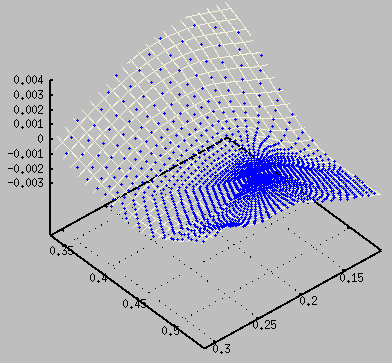
The plot shows a zoomed in section of the HSM LUT (blue dots) and the native LUT (beige grid).
  splot \
    'nve-lut.dat' w l lc "beige", \
    'hsm-lut.dat' pt 1 lc "blue", \
    'gmt-prophoto.dat' w l lc "red", \
    'gmt-locus.dat' w l lw 4 lc rgb var
The HSM LUT operates in linear Prophoto RGB space, converted to HSV. This means that in an u'v' coordinate system it looks very dense close to the white point, and then becomes gradually less dense, clearly seen in this plot.
While DCamProf's native format is 2.5D, the color space is different
from the DNG profile and DCamProf also adds a subtle 3D gamut
compression step for the extreme range.
This means that it's not possible to get an exact match with a DNG
2.5D HSM LUT. However the difference is very small, and also the gamut
compression from the extreme range will translate well (although
look slightly different) so therefore the HueSatMap is suitably kept at
2.5D to keep down the profile size. You can force it to make a 3D
table though, using the -D flag.
Manual edits
When running the make-dcp command you can specify many but not all
tags. If you want to adjust some of the remaining tags you need to dot
this manually by using the dcp2json and json2dcp
commands:
- Convert the DCP to human-readable JSON format.
dcamprof dcp2json input.dcp dcp-profile.json
- Manually edit
dcp-profile.jsonusing a text editor. - Convert the JSON file back to DCP.
dcamprof json2dcp dcp-profile.json output.dcp
Dual-illuminant DNG profiles
To make a dual-illuminant profile two separate native profiles are made (one for each illuminant) and then both are passed to make-dcp, like this:
dcamprof make-dcp profile1.json profile2.json dual.dcp
The lower temperature illuminant should be listed first, and you must
have illuminants with known temperature, ie you cannot have "Other"
which the profile will have if you have used a custom calibration
illuminant. If so, specify illuminants using the -i and -I parameters.
As the DCP profile format only supports pre-defined EXIF light sources
pick out sources that as close as possible matches the temperature of
your custom illuminants.
Note that the light source temperature is the only thing that matters to DNG profiles, it makes no difference if it's a fluorescent (peaky spectrum) or tungsten (halogen, smooth spectrum), so if your calibration illuminant was a 3500K halogen lamp, the EXIF light source "WhiteFluorescent" (3525K) is the best choice.
DCamProf makes no sanity check on your illuminant listing so if you use "Other" or place the highest temperature light source first the resulting profile may not work as intended in your raw converter.
The most common dual-illuminant combination in commercial profiles is StdA and D65. It generally makes little sense to combine say D50 and D65 as they're so similar. The general idea of dual illuminant profiles is to make a generic profile that works in varied light conditions, and then you want to combine two light sources whose white points are relatively widely spaced. Look at the color temperatures plotted in a chromaticity diagram for example to get and idea of how much they differ.
D65 is considerably harder to simulate (well) than D50 in an indoor profiling setup. Fortunately the combination of StdA and D50 still provides a wide spacing between light sources and is a good alternative to the more common StdA + D65.
Avoiding white balance shift
If you have used a previous profile and custom white balance in your raw converter, applying your new profile will likely cause a white balance shift. See the section on DCP-specific white balance properties for a description why this can occur.
If you want to avoid this you need to replace the color
matrix/matrices in your new profile with those found in the old, by
using the -m parameter. As color matrices are only used for
whitepoint temperature calculations and no actual color corrections
this will not affect color rendition for single-illuminant
profiles. The ability to predict white point color temperatures is in
full replaced by the old profile though, and due to that a
dual-illuminant profile will render color (very) slightly different as
the derived temperature is used when mixing the forward matrices and
HSM LUTs for the color correction step.
When making a profile to be used as drop-in replacement to a raw converter's bundled profile, it's generally a good idea to use the bundled profile's color matrices to avoid this white balance shift.
Tone reproduction
If you're making a profile for reproduction work you should not apply any curve, likewise if the targeted raw converter is designed for linear colorimetric profiles (scene-referred profiles). This is the default. However, most raw converters expect general-purpose profiles to apply a contrast-increasing "film curve", and in the case of DNG profiles this curve is embedded in the profile itself.
Per default DNG raw converters use a type of RGB curve that has some
color distortion issues as discussed in
the tone curves section. DCamProf can
instead apply an own curve type (via 3D LookTable corrections) which
is more neutral. This is enabled per default (controlled by the -o
parameter), but will only be used if a curve is applied (-t
parameter). The properties of this is discussed in the section
about DCamProf's neutral tone
reproduction operator. You may also want to read
the DNG profile implementation notes
regarding this before using it.
The supplied curve is either one of the built-ins, linear, none,
or acr (Adobe Camera Raw's default curve which is a good choice in most
circumstances), or a custom curve in a JSON file, or a RawTherapee
curve file (.rtc).
The JSON file format can be the same as for the
transfer function, but only the GreenTRC tag will be used, or TRC
or GrayTRC if those are available. You can also provide a
ProfileToneCurve from a DNG profile in JSON format. As
usual all other tags are ignored so you can provide a full JSON of a
DNG profile (as produced by the dcp2json command).
The RawTherapee .rtc format is supported, but only for "Spline" and "Linear" curves. It's a simple text file format with XY handles for spline or linear interpolation in sRGB gamma (both X and Y axes are gamma-scaled). See the data-examples directory for an example. If you wish you can design the curve using RawTherapee and export it from there. The "Linear" type is suitable if you generate a curve with hundreds or thousands of handles, then they are interconnected with linear segments.
The available tone reproduction operators are
the "neutral" operator, and
"standard" operator which in the DNG profile case means just embedding the
curve and make no change in the LUTs, and then the raw converter will likely apply
an RGB type of curve. Instead of "neutral" or "standard" keywords you
can provide the name of a JSON file that contains custom weights for
the neutral tone reproduction operator. See
the ntro_conf.json file in the data-examples directory
for further details. Normally you should not need to provide custom
weights, but should for example the auto curve analysis lead to a too
large or small chroma scaling factor you can set it manually using the
configuration file.
Some raw converters are meant to be used with colorimetric profiles without any curve, but may still not have any good tone reproduction operator built-in, meaning that it will be very hard to achieve realistic colors as soon as you apply contrast. In that case it may still be worthwhile to apply the tone reproduction in the profile, if the raw converter supports both ways (which is the common case).
Gamut compression
As a part of the neutral tone reproduction operator you can optionally configure gamut compression. There's a commented configuration example in the data directory which serves as the main documentation.
The purpose of the feature is to compress the gamut so super-saturated colors fit into a smaller gamut. It's typically used to make sure the profile doesn't output colors more saturated than sRGB or AdobeRGB. This is the "gamut mapping" feature, but as it's always used to compress from a larger to a smaller gamut and is much less complex than mapping to a printer's irregular gamut (the usual application for gamut mapping) it's called "gamut compression" here.
The gamut compression is generally configured such that some clipping is allowed, otherwise transitions into saturated highlights (sunsets etc) will look dull.
Although I'm personally not a fan of gamut compression, most bundled profiles have it and few raw converters have good automatic gamut compression so if you shoot lots of saturated colors (such as flowers) and want good tonality straight out of camera without having to fiddle with manual adjustments, it's generally a good idea to apply some gamut compression in the profile.
Instead of specifying the gamut compression in the neutral tone
reproduction configuration file you can provide presets directly on
the command line using the -g parameter. Using
-g adobergb-strong is a good start if you want to
try it out. It may seem odd to start out with a "strong" compression,
but bundled profiles usually have quite strong compression so if
you want similar results this is it.
DCamProf's gamut compression is not designed to make a mathematically exact compression such that exactly no clipping takes place, as this actually won't look any good. Some clipping needs to take place to avoid dullness, especially of subjects that clips the actual raw colors such as sunsets.
Documentation on how the gamut compression algorithm works and how it can be precisely configured is found in the look operators example configuration file in the data-examples directory.
Designing a subjective look
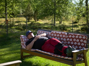
An example image rendered with a neutral profile. It's a colorimetric accurate base profile, with a contrast S-curve and DCamProf's neutral tone reproduction operator on top.
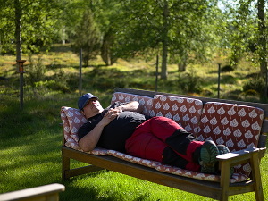
Same image but here with a designed subjective look. Without layering the image on top it will be difficult to see any difference, and this is how it should be. A successful designed look is typically very close to neutral. The most visible change in this look is that yellows and greens have been warmed up.
You can extend the configuration file for the tone reproduction operator with "look operators". The purpose of these is to design a subjective look which is applied on top of the neutral tone reproduction.
Be warned that this is not an easy task, especially since DCamProf lacks a graphical user interface. The process of designing a look means rendering lots of profiles with minor adjustments and comparing until you are satisfied with the result. It requires that you have a good eye for color and know what you want to achieve.
The intention of DCamProf's "look operators" is to make very subtle adjustments, small deviations from the neutral look. That is it's not intended to make strong "filters" like simulating cross-processing, fading or other effects related to analog photography.
Look operators key concepts:
- The array of look operators are applied after the tone reproduction operator.
- The look operators are applied in order one after another, so the order matters.
- With a "Blend" array inside each look operator you define which part of the gamut it should be applied and how it should be be blended in.
- Main color space is CIECAM02 JCh, Lightness, Chroma, Hue, but you have also access to RGB space(s) with ProPhoto primaries.
- You can change the color of neutrals with the operator, but it will only work for ICC profiles (DNG profiles doesn't support it by design), so if you design for DNG make sure you blend out the effect towards the neutral axis (if needed).
As already touched upon it will be very difficult to drastically change the look and get good results, so if you not at all like how DCamProf renders colors in it's neutral mode you are in trouble, as the adjusted profile will typically still be quite close to neutral. In that case I suggest using some other software as DCamProf is foremost about neutral and realistic color rendering.
Available look operators:
- AddHue
- Note that the "Curves" operator is typically more useful when you want to modify hue.
- AddLightness
- AddChroma
- ScaleChroma
- ScaleLightness
- SetTemperature
- Used to warm up or cool down. A common adjustment is a slight warm-up of midtones and highlights while cooling down shadows.
- 5000K tint 0 is always the reference temperature (=no change), lower temperatures will cool down, higher will warm up.
- Curves
- RGB curves operating with ProPhoto primaries, can be used for traditional skin tone tuning using RGB/CMY curves.
- User-selectable gamma by number, or specify "sRGB" for sRGB gamma.
- Stretch
- Compress or expand in one to three dimensions (CIECAM02 JCh). Usually this is used in the hue dimension to either reduce hue spread or increase it in some range.
- You can use it to even out skin tones for example.
As there is no GUI you need to work with trial-and-error. Using a raw converter that quickly and effectively can load new profiles (like RawTherapee) is highly beneficial. To see what colors that will be affected in an image (that is what area the "Blend" section covers) a good alternative is to use "ScaleChroma" with "Value" 0 and as then all colors covered by the blend will be monochrome (set "BlendInvert" to true if you want the inverse).
For example if you want to target skin tones you adjust the "Blend" section so only the faces become monochrome, and then you can use this selection for various adjustments in the real profile.
Curves are used in blending, and in the "Curves" and "Stretch" operators. There are three type of curves: "Linear", "Spline" and "RoundedStep". The "RoundedStep" is just a step function with S-curve transition, the other two are self-explanatory. Be warned that it's difficult to design a spline in the blind as it easily suffers from overshoots. You can test curves in GNUPlot or design curves in RawTherapee. The RGB curves operator can be mirrored exactly in RawTherapee by selecting ProPhoto working space, and in the operator select "sRGB" gamma. Then you can design the curves operator look in RawTherapee, export the curves, open in a text editor, reformat and put it in your JSON file.
When blending in various look operators there is a risk that you disturb the overall smoothness of the profile, perhaps you're making too strong adjustments with a too narrow blending zone. An effective way to diagnose this is to use the test-profile command and dump and image with processed gradients.
To see how the syntax works and get further documentation, look in the data-examples directory where you can find a documented example.
Hue shift discontinuity
The DCP LUT works in RGB-HSV space, which means that the hue is defined as an angle 0 to 360 degrees, and modifications to the hue is defined as an offset to the input hue angle.
When the input hue angle falls in-between two LUT table entries the offset is interpolated. For example if entry A says "add +40 degrees" and entry B says "add −30 degrees" and the input angle falls exactly in-between the average is calculated as "(+40 + −30)/2 = +5 degrees".
If we have a large hue shift say going from +170 to −170, the actual difference between those to neighbors is only 20 degrees and the average would be ±180, but most DNG pipelines (probably all) don't support hue shift discontinuity and simply calculates this as "(+170 + −170) / 2 = 0". I would like to call this a bug, as hue angle discontinuity is a well-known caveat when working with these type of coordinate systems, something that well-designed code handles without issues. The discontinuity is just in the math (it must wrap around somewhere), not in the actual hue transition.
Unfortunately Adobe's DNG reference code doesn't handle the wrap, and thus probably all software supporting DNG profiles doesn't either. Therefore make-dcp will per default abort if it detects a hue shift discontinuity.
Fortunately it's very unlikely that a discontinuity would occur in a normal colorimetric profile. It can quite easily happen when you design a subjective look with look operators though, and the solution is then generally to fade out the operator on the "HSV-Saturation" axis.
The built-in DNG pipeline in DCamProf uses the DNG reference code and will thus cause discontinuity artifacts just like the others. This means that you can see discontinuity artifacts when dumping a test gradient.
Observer remapping
DNG profiles has linear Prophoto as a working space, which is defined with the 1931_2 observer. That is raw converters using DNG profiles expect the D50 whitepoint map to D50 of 1931_2. If you have used a different observer you will get slightly different XYZ values, and the D50 whitepoint will thus have a slightly different coordinate. There may be a 1–2 Delta E difference.
Many raw converters sanity-check the profiles to see that the whitepoint in the forward matrix matches 1931_2 D50, and if not they consider the DCP invalid and refuse to load it.
Therefore DCamProf will also do this check and if it detects a different whitepoint it assumes a different observer has been used in profile making, and adjusts the matrices and LUT-making with a linear Bradford transform to adapt.
This transform is certainly not perfect when it comes to transform from one observer to another, and as discussed in the observers section it's not recommended to use any different observer than the default 1931_2 for production profiles.
As the default observer is 1931_2 this remapping will only take place if you have changed the observer when making the profile. If you want to compare errors you can run a test-profile on both the native profile and the resulting DCP. The native profile will not need observer remapping. Note that the mapping from the native LUT to the HSM LUT will also generate slight differences from the native profile. Make sure you provide the desired observer in test-profile too, otherwise you will see large errors.
The color matrix is not remapped. It's only used for illuminant temperature estimation and as the difference between observers is way smaller than the error you can expect in the estimation it's kept as is.
Examples
Basic conversion (replace the name with your specific camera name):
dcamprof make-dcp -n "Canon EOS 5D mark II" profile.json profile.dcp
Dual-illuminant profile with the illuminants specified (overrides tags in source profiles):
  dcamprof make-dcp -n "Canon EOS 5D mark II" -i StdA -I D65 profile1.json \
    profile2.json profile.dcp
dcp2json, json2dcp
  dcamprof dcp2json <camera.dcp> [<dcp.json>]
  dcamprof json2dcp <dcp.json> <camera.dcp>
Convert DCP profiles to and from JSON format, useful for making manual edits of individual tags.
make-icc
dcamprof make-icc [flags] <profile.json> <output.icc>
Converts a profile in DCamProf's native format to an ICC profile which can be used directly in various raw converters. Note that ICC profiles that works for one raw converter may not work in the next as the color rendering pipeline is not standardized.
Overview of flags:
-n <camera name>, actually the ICC "description" tag, may contain what you like but camera name is a good idea.-c <copyright>, the copyright tag string. If spaces in the string, provide within quotes.-s <CLUT side division>, how many divisions the LUT cube side should be divided in, default is 33.-p <lablut | xyzlut | matrix>, profile type (default:lablutif input has LUT otherwisematrix).-L, skip LUT of input profile, the output profile can still contain a LUT if you force it with the-pparameter.-W, let the profile correct white balance, usually not desired except in some specific reproduction setups.-f <file.tif | tf.json>, adapt the ICC profile to match the transfer function in provided TIFF / JSON, only required for raw converters that apply a curve to the raw data before applying the profile.-t <none | acr | custom.json>, apply a tone curve to the LUT. For colorimetric accuracy you should have no curve. To apply a default film-curve, which may yield a more pleasing look, chooseacr. You can also supply a custom curve. Note that the tone reproduction operator (-o) will affect how this curve is used. Default:none. Curves can be cascaded, that is you can provide-tmore than once.-o <neutral | standard | custom.json>, tone reproduction operator (default:neutral). Will only be applied if a non-linear curve is applied (-tparameter).-g <none | srgb | adobergb | srgb-strong | adobergb-strong>, gamut compression presets. Will only be applied if curve is applied (-tparameter) with the neutral tone reproduction operator. You can configure the gamut compression more precisely in a tone reproduction operator configuration file (-oparameter). Default: none (or from the configuration file if any).-T, don't apply tone curve to the LUT. Used if the raw pipeline will apply an RGB curve after the ICC profile is applied. Note that this is not common, if the raw pipeline applies a curve separate from the ICC it's normally done before the ICC is applied.-r <dir>, directory to save informational reports and plots.
Compatibility
While ICC profiles in general are rigidly standardized, it's not well standardized how camera ICC profiles are applied in raw converters. They are often not applied directly to a linear raw image like DNG profiles always are, but rather there is some extra pre-processing step before, and possibly a post-processing step after. This means that ICC profiles are not possible to move between different software in the same way as DNG profiles. You may need to design your ICC profile specifically for one raw converter.
My intention is that DCamProf should support all reasonably popular raw converters, and I think it already does but I haven't tested them all. If you find any compatibility issue let me know. I cannot promise I will implement support for every ICC-using raw converter though.
DCamProf supports raw converters which either provide demosaiced linear raw data as input to the ICC (like for example DxO Optics can do), or the same with a curve (like for example Capture One does). If a curve is applied that must be taken into account during the workflow. See the ICC example workflow for further information.
White balance
Most (probably all) ICC-using raw converters will apply the camera's white balance before the ICC profile is applied. You can see this if you export a file for profiling, if the white balance seems applied, then it is.
Still, a camera's "as shot" white balance rarely matches the calibration illuminant exactly, that is a perfectly white patch will not be be rendered with R=G=B, but instead have a slight tint. DCamProf which knows the the XYZ coordinates for each patch and thus what white should be can correct for this if desired. However, this would mean that when the profile is loaded the white balance will change so a perfect white (rarely exists in the target so it's interpolated) becomes RGB 1,1,1. This might be what you want, but likely not. Probably you want to keep the camera's original white balance and therefore this is the default when DCamProf makes ICC profiles. DCamProf will simply make sure that the profile maps camera white-balanced raw RGB 1,1,1 to D50, that is use the native forward matrix mapping as is.
Note that since DCamProf normalizes the white balancing when making it's native profile it doesn't matter which white balance the test image had. This means that you can convert the same native profile to both a DCP and an ICC profile, even when it was made from non-white-balanced data (like DCP requires).
Are there cases when you do want the ICC profile to correct the white
balance? Yes, for example in a fixed light reproduction setup when you
want to use a white balance preset on the camera (easy to remember and
recall) but still get as correct white balance as possible in the
final image, then the ICC profile should correct it. To do so supply
the -W flag when making the ICC. For this to work the
native profile must have been made from a white-balanced test image
though (using the camera's preset of interest).
ICC profile type and ICC LUTs
DCamProf can make a pure matrix profile (with shaper curves if
a transfer function is provided via the -t parameter),
and a LUT profile with either camera RGB to XYZ conversion or camera
RGB to Lab.
By specifying the type you can make a LUT profile even if the input doesn't have a LUT, which may be useful for testing in some cases.
An ICC LUT is always 3D, a table with RGB triplets as input and corresponding XYZ or Lab triplets as output. Ideally you would have a table entry for all possible RGB combinations which would be 65535³ for 16 bit data, but that would fill your hard-disk with just the ICC profile so it's not a good idea. Instead the range is coarsely split (33 is default) and the inbetweeners are interpolated.
DCamProf generates the ICC 3D LUT by sampling the native LUT (and the tone reproduction operator if used), and applies an input curve to get better perceptual spacing of the LUT cube divisions. ICC LUT resolution can at times be a problem. If you do get problems matching some patches you can try increasing the cube divisions from the default 33. Be warned though that the size of the ICC file will grow very quickly with increased number of divisions. A reasonable test value is 128 which will yield a 12 megabyte ICC profile, and then reduce from there towards the default 33.
DCamProf can make an RGB to XYZ or an RGB to Lab LUT, the latter is the default. Currently the XYZ LUT uses the forward matrix directly which means that extreme value handling is not as good as the Lab LUT, so I recommend using the default Lab LUT.
Tone reproduction
The tone reproduction functionality is largely the same as described for DNG profiles, I recommend reading that first. The difference is that ICC profiles don't embed a separate curve and look table, so the tone reproduction curve will be applied directly in the sole ICC 3D LUT.
Many ICC raw converters apply a curve on the side though (for example Capture One), and in that case you should employ the raw converter's linear curve during profiling and again when using the finished profile, as the LUT in the profile itself will take care of the tone reproduction curve. However there are other ways to do it as well, you can read more about Capture One specifically in the Capture One and curves section.
If you want to apply a subjective look you can do so, as documented in the subjective look design section. A difference from DNG profiles is that ICC profiles will allow you to change the color of neutrals.
You can also enable gamut compression.
Plotting ICC LUTs
You can add the -r <report_dir> flag to
get report files which include ICC plot
files. As ICC LUTs are 3D they are a bit cumbersome to visualize. You can
plot all points in the 3D LUT "cube" by plotting icc-lut.dat,
but it may be better to plot a slice at a time using
the icc-lutXX.dat files. The main thing to look for is if the
LUT seems dense enough to replicate the stretching that is in the
native 2.5D LUT. It shouldn't have overkill density either as
that will make the ICC file larger than needed, especially since LUT
ICCs are always a bit large due the 3D LUT.
Plotting the full 3D LUT with error vectors and target:
  splot \
    'icc-lut.dat' w d lc "beige", \
    'gmt-locus.dat' w l lw 4 lc rgb var, \
    'gmt-adobergb.dat' w l lc "red", \
    'gmt-pointer.dat' w l lw 2 lc rgb var, \
    'target-icc-lutve.dat' w vec lw 2 lc "black",\
    'targetd50-xyz.dat' pt 5 ps 2 lc rgb var
The example shows the default LUT with 33x33x33 points, it still becomes very dense in a 3D plot. The sides of the "gamut" are quite sharp and the shape is boxy, this is because the LUT reaches the full range defined by the LUT table and clips there (this is outside the real color range though, so don't worry).
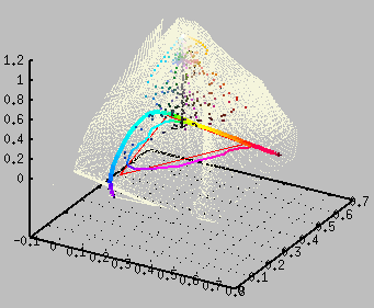
The same plot as above, but now with just a slice:
  splot \
    'icc-lut10.dat' w d lc "beige", \
    'gmt-locus.dat' w l lw 4 lc rgb var, \
    'gmt-adobergb.dat' w l lc "red", \
    'gmt-pointer.dat' w l lw 2 lc rgb var, \
    'target-icc-lutve.dat' w vec lw 2 lc "black",\
    'targetd50-xyz.dat' pt 5 ps 2 lc rgb var
There are 20 slices indexed 00 to 19, here we plot index 10 which means 0.5 to 0.55 in the native LUT lightness range (which is Lab lightness scaled to 0.0 – 1.0 range).
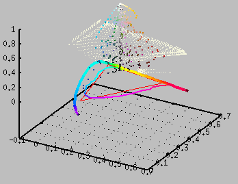
The same plot as above, that is a LUT slice with target and error vectors, now viewed straight from above and zoomed in on a detail around skin-like colors.
We see here that the profile is less accurate on darker colors (longer error vectors), while spot on on the brighter. The beige crosses show the LUT points in the slice. They are here in close-by pairs as the slice fits two levels (look from the side to see), so for the actual "2D" density think of the nearby pairs as one point.
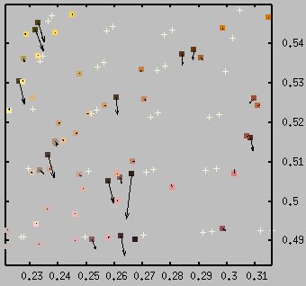
icc2json, json2icc
  dcamprof icc2json <camera.icc> [<icc.json>]
  dcamprof json2icc <icc.json> <camera.icc>
Convert ICC profiles to and from JSON format.
ICC is a large standard and supports many types of devices in addition
to cameras, such as printers, scanners and monitors. DCamProf's ICC
parsing is only focused on ICC version 2 camera profiles, and will
ignore any irrelevant tags and refuse to parse ICC profiles that aren't
camera profiles. The commands are intended for looking at and editing camera
profiles, no other ICC types. This means that icc2json does not
work well as a generic ICC dis-assembler. If you really need to see all
tags in an ICC Profile you can for example use
Argyll's iccdump tool.
tiff-tf
dcamprof tiff-tf [flags] <target.tif> [<transfer-function.json>]
Extract the transfer function (TIFFTAG_TRANSFERFUNCTION)
from a TIFF file and write it to a JSON file. The transfer function is
a linearization curve, that is if the data has been made non-linear
by a tone curve the transfer function will be the inverse of that tone
curve.
The extracted transfer function can then be used in other relevant commands such as make-icc to linearize data. As make-icc and make-dcp can take the TIFF file directly extracting it first is generally only for informational purpose.
You can however also calculate a tone curve using this command (as the difference between two transfer functions), which cannot be done with any of the other commands.
Overview of flags:
-R, skip reconstruction. The transfer functions are defined using integers and often there are several entries in a row with the same number due to the rounding. Per default DCamProf will reconstruct those values with a robust linear interpolation. If you don't want that to happen you provide this flag.-f <linear.tif | linear.json>, reference TIFF / JSON with the transfer function corresponding to linear response. This is then used to convert the provided TIFF to a tone-curve in linear space rather than a transfer function.
Some raw converters, like Capture One, applies the tone curve before
the ICC profile. If you want to extract that tone curve to use in a
DCamProf workflow you need to remove the transfer function for the
linear component. You then do the following: export one TIFF with
linear response linear.tif, and one with the desired curve
curve.tif, and then you run the command:
dcamprof tiff-tf -f linear.tif curve.tif tone-curve.jsonThe output will then contain a tone curve in linear space calculated by applying the transfer function from
linear.tif to the inverse of
curve.tif. This tone curve can then be provided to make-icc or
make-dcp with the -t parameter.
txt2ti3
dcamprof txt2ti3 <input.txt> <output.ti3>
Import spectral data from a text file, further described in the make-target section.
make-testchart
dcamprof [flags] make-testchart <output.ti1>
Generate an Argyll .ti1 file (like Argyll's
own targen) that can then be used with
Argyll's printtarg command to make a test chart that can be
printed.
Overview of flags:
-p <patch count>, choose number of patches to generate, default is 100.-w <percentage white patches>, specify the percentage of white patches. The target will be speckled with white patches which then can be used as anchors for flatfield correction. Default: 20%.-b <black patch count>, black patches doesn't really contribute to profiling, but is good to have a few for sanity checking contrast and exposure, as well as allowing glare matching. The default count is 5 which will be evenly spread out over the target.-g <gray steps>, if you want a linearization step wedge specify here how many in-between gray levels there should be. The number of gray patches on each level is the same as the black count.-l <layout row count>, specify the intended row count of the target. Specifying layout is required if you want an optimal white patch distribution.-d <layout row relative height>,<column relative width>, relative width and height of patches, you can specify it in any unit you like as it's only relative. Default: 1,1 (square patches).-O, specify this flag if the chart layout has even columns offset a half patch. Argyll'sprinttargmakes Colormunki style targets this way.-r <dir>, directory to save informational reports and plots.
This command is basic, it only supports RGB output (as most inkjet printers today are controlled as pseudo RGB devices), and you can only control the patch count, not which patches that are generated. The patches are generated such that it starts with one white patch, and then patches are spread out with as long perceptual distance as possible, with the constraint that only the lightest possible color of a certain hue and chroma are used. That is there will for example be no brown patch, as brown is actually dark orange. The rationale behind this is that as the LUT is 2.5D it's only necessary to profile the lightest colors, as any darker colors would be grouped together in a chroma-group anyway.
The patch placement in terms of perceptual distance will not be perfect as the command is unaware of the printer's profile, but as the coverage is intended to be dense it doesn't matter.
Today's inkjet printers typically have more colorants than older models, which means that the spectra can be a bit more varied. However the spectral variation will still suffer compared to commercial test targets made with special printing techniques. Your mileage may vary.
The test chart generator's intention is to fill the gamut so it will need quite many patches to not miss out any corner. 50 patches is probably more than enough, but if you're printing an A4 sheet you could just fill it even if it will be a bit overkill. You can increase the white patch percentage to save ink.
With the -b and -g parameters you can add step wedges for
linearization. This might be an advantage for targets that will be
shot in situations where glare can be an issue.
testchart-ff
  dcamprof testchart-ff [flags] <input.ti1 | layout.json> \
    <input.ti3> [<input2.ti3>] <output.ti3>
...or
dcamprof testchart-ff <input.tif> <flatfield.tif> <output.tif>
Either flatfield correct .ti3 data or a linear TIFF file. If you're
correcting a .ti3 file it must be a target speckled with white patches
and the layout must be specified via a .ti1 file and the layout
flags, or a layout in JSON format (a documented example exists in the
data-examples directory). If you are correcting a TIFF file the input
files must be 16 bit in linear gamma.
It's also possible to model glare, this requires a neutral step wedge in the file, or even better neutral patches (black, white and middle gray) spread out over the whole surface.
Overview of flags:
-l,-d, and-Olayout specification flags working in the same way as for the make-testchart command.-L, enable glare matching.-r <dir>, directory to save informational reports and plots.
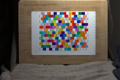
If you shoot indoor and have only one light it's difficult to get even illumination of the target. In this example the difference between the lightest and darkest white patch is as much as 1 stop. The flatfield correction algorithm uses all the white patches as anchors and makes one thin plate spline surface per channel to correct. While I recommend to have more even light than shown here, this will work.
Animated image showing the result of a profile made with glare matching and one without, designed from the actual shot of the ColorChecker SG semi-glossy target shown in the picture.
At first glance the target may look well-lit and without issues, and indeed the white patches along the border are all equally bright, indicating perfectly even illumination (no need for flatfield correction here!). However look at the black patches, the ones along the right border are considerably lighter than the ones on the left. This is not due to uneven illumination, the neighboring white patches are the same brightness, the problem is instead glare. The target thus get lower contrast on the right side where there is more glare than on the left.
The animated images shows what happens if you make a profile ignoring the glare. Look at the dark red-purple patches in the top right corner. They become much darker with the uncorrected profile. The reason is that the make-profile gets much brighter camera raw samples than it should (affected by glare) and thus makes a profile that darkens them heavily to compensate.
Glare lowers contrast affecting dark colors the most, and as the resulting profile will compensate the result will be opposite, too much contrast and too high saturation.
The left side has much less glare and thus the colors change less between the two profiles. However if hue is shared with a patch on the heavily affected side there is still a strong effect which can be noted in the pink patch in the CC24 section of the target. Note that the animated GIF image is limited to 256 colors so the more subtle differences cannot be seen.
The ColorChecker SG target is interesting as it's one of the few commercial targets that has white/black/gray calibration patches along the border of the target. DCamProf makes use of this and thus both flatfield corrects and makes a locally varying glare matching. This way the right side patches have been much more strongly corrected than those on the left side.
While a good result is had with this shot, I strongly recommend against relying on glare matching. Instead make a proper setup which has less glare than shown in this example. It's much more important to minimize glare than to have even illumination, as flatfield correction can even out the differences precisely without adverse effects, while glare matching by nature has to rely on an imprecise model.
If you have made sure to illuminate the target evenly and done it well the difference of applying flatfield correction will be negligible so it's certainly not mandatory. If you shoot a large target indoors and have only one light it's however most likely that you need to flatfield correct.
If your target is speckled with white patches you don't need to shoot
an extra flatfield shot, correction can be made directly on the .ti3
data. When the target is photographed we know that if the lighting is
perfect all white patches should give the same RGB values. Light is
never 100% uniform though so the white patches will vary. Based on the
positions of those white patches and the variations thin plate spline
correction maps are created to scale all patch values to match uniform
illumination.
The indexes of white, black and gray patches are found out from the
provided .ti1 file. If you have used the make-testchart command you
have already such a file, if not you're better off making a
target layout JSON file, look in the data-examples directory to find a
documented example. For flatfield correction you only need to point
out the white patches.
Most commercial targets are not speckled with white patches though,
and then you need to pre-process the TIFF file before
you feed it to Argyll's scanin. First shoot the target, then with the
exact same lighting place an equally large or larger white card in the
exact same position as the target, and shoot it from the exact same
camera position. Then make the exact same crop/rotation of both files
and export to linear 16 bit TIFF. The image must be cropped enough so
that only the white section of the white card is visible, if any
surroundings or edges of the card is visible the result will not be
good.
Feed those TIFF files to the testchart-ff command and you will get a
new flatfield corrected output file which you then can feed to
Argyll's scanin.
Another alternative is to print a chart with only white patches (ie
only a grid) that exactly matches the target you have, and swap in
that in a second shot (light and camera setup must be stable of
course). You then run testchart-ff with this extra .ti3 file, so you
have first the layout .ti1 file (showing only whites in this case),
the white target .ti3, and then your real target .ti3 and finally the
output .ti3 file. This may be a bit cumbersome way to apply flatfield
correction, it's probably considered easier to shoot a gray or white card
instead and pre-process the TIFF file.
There are specific white card products to buy, but these are quite expensive. Instead you can for example use an unprinted high quality photo paper (without see-through). I recommend a smooth matte OBA-free paper, make sure it lays perfectly flat just like the target. It does not matter if the card is slightly off-white, in theory it could be any color as flatfield correction just corrects differences from the global average.
Glare matching
Many targets contain a neutral step wedge that can be used to linearize the raw samples to compensate for glare. However this process is hard to get stable and robust so DCamProf has chosen a different approach: add glare to the reference values (or spectra) so it matches the camera's raw samples. This process is called "glare matching".
That is instead of removing glare from the raw samples, we add glare to the reference data. As DCamProf knows the response of the observer (unlike the camera) it can apply certain robustness features to the glare model. The problem with glare modeling is that unlike flatfield correction it cannot be very precise. There are too many unknown factors, so DCamProf must rely on very coarse models. With more advanced models there's a large risk the result gets worse due to that there's too little input data to feed the models with.
In DCamProf's glare matching algorithm robustness is a main priority, that is don't make it worse than it was from the beginning. For example the glare matching will not alter hue, only lightness and chroma.
You can enable glare matching with the -L flag. It only works
on .ti3 files, so if you have a TIFF you can flatfield it first, then
scan it and then glare match the .ti3 file by running this command
again. A flatfield pass is always run first (if possible).
I do recommend to do everything you can to minimize glare at shooting time. While it's perfectly ok to rely on flatfield correction, as it can accurately even out illumination, it's not a good idea to rely on glare matching as modeling can't be as precise.
It may still be worthwhile to run glare matching even if you have minimized glare during the shoot as it's almost impossible to eliminate it in full. With small amounts of glare in the original shot the glare matching algorithm makes better results than it can with large amounts.
If you run with a report directory (-r parameter) you will
find glare-match.tif there which shows how the reference
patches were adjusted to match the camera glare.
average-targets
dcamprof average-targets <input1.ti1> [<input2.ti3> ...] <output.ti3>
If you have problems with too much noise in the darkest patches in
your test target photos, you can make multiple shots, convert all to
.ti3 files and then average them using this command. Averaging shots
is an alternative to classic HDR merging and has the advantage that
all shots are fully usable and thus scannable by
Argyll's scanin command.
You can do averaging/merging of images in other software too
and make a new image which you then feed to Argyll's scanin,
however you must then be absolutely sure that the software produces
100% linear results and that is often not the case.
In most circumstances there is no need to average several shots, the noise in one shot should be low enough if properly exposed.
match-spectra
  dcamprof match-spectra [flags] <reference.ti3> <match.ti3> <output-match.ti3> \
    [<output-ref.ti3>]
Find the spectra in match.ti3 that best matches the spectra
in reference.ti3, either as seen by an observer or by camera
SSFs.
Overview of flags:
-o <observer>, observer for DE comparison, default 1931_2.-i <test illuminant>, the illuminant the comparison is run under, default D50.-c <ssf.json>, camera SSFs, if provided these will be used instead of the observer for patch spectrum comparison, and then Euclidean distance is used as error value instead of CIEDE2000.-S, scale spectra (that is adapt lightness) in output to better match the reference spectra.-N, normalize patches before comparison, meaning that a dark can match a light patch if the spectral shape is the same.-U, don't allow repeats of the same spectrum in the output. That is if the best match for a given patch is also the best for another it's still written only once to the output.-E, consider all spectra as emissive. DCamProf supports a tag in the.ti3files that specifies if the patch spectrum is emissive or not. This flag causes the tag to be ignored, and all spectra is considered emissive, that is they will not be integrated with the test illuminant.-e <max DE>, maximum acceptable DE to consider it to be an acceptable match, default is infinite that is the best regardless of error is included.-r <dir>, directory to save informational reports and plots.
This command is typically not used in any profiling workflow, but is instead used for informational purposes. You can for example test how well the "skin-tone patches" of your commercial target matches real skin-tones from a spectral database.
As DCamProf's camera profiles are 2.5D it often makes sense to scale
lightness to match, both when comparing (-N) and when outputting (-S). If you
specify one output it will contain spectra from the match.ti3
that matches, and if you specify two the second output will contain
the patches from reference.ti3 for which an acceptable match
was found. Per default there's no error limit and non-unique matches
are allowed and then the second output will be a copy
of reference.ti3. Add parameters to narrow down the matching.
If a report directory is given (-r), spectra and XYZ coordinate plots
for inputs and outputs are stored there.
si-render
dcamprof si-render [flags] <spectral image> <output.tif>
Render a normal RGB TIFF from a spectral image, specifying illuminant and observer or camera SSF.
Overview of flags:
-i <illuminant>, the illuminant to light the spectral image with, default D50.-o <observer>, observer, default 1931_2.-c <ssf.json>, camera SSFs, if provided these will be used instead of the observer.-g <gamma>, gamma in output, default 1.0. Note that a gamma of 1.8 is required if the output should be processed by the test-profile command.-W, apply white balance.-b<base band>[,<band width>], specify base band and width for indexed files.-P, enable ProPhotoRGB output.-a <bradford | cat02>, choose CAT (output space is D50 in this case).
The spectral image format must either be the SPB format or a directory with normal monochrome TIFF files with spectral band (in nanometers) in the filenames. An example image with this format is the METACOW test image from Munsell Color Science Laboratory.
For the SPB format description and links to example files you can go to the www.multispectral.org web site.
Spectral images can become very large and DCamProf will read it all into RAM memory, so make sure you have enough.
While you can use this to just test differences between observers or CATs, the typical use case in camera profiling is when you have camera SSFs and want to test how camera profiles react under different light. You then render "virtual raws" with your desired illuminant and camera SSF using this command, and then you process that through the profile by using the test-profile command:
  dcamprof si-render -c 5dmk2-ssf.json -W -g 1.8 -i D65 input.spb test.tif
  dcamprof test-profile -c 5dmk2-ssf.json -i D65 test.tif 5dmk2.dcp output.tif
Report directory files
When DCamProf is run with the -r <report_dir> parameter
enabled it will write data files for plotting, report text and image
files. The plot data files are suitable to plot
with gnuplot, but you can use
any other plotting software if you like as the data is stored in plain
text files.
Text files
The report text files contain patch matching reports:
cm-patch-errors.txt, color matrix patch matching errors.fm-patch-errors.txt, forward matrix patch matching errors.patch-errors.txt, patch matching with full LUT correction (if any).
A patch matching row looks like this:
A1 RGB 0.076 0.095 0.040 XYZref 0.130 0.113 0.057 XYZcam 0.129 0.112 0.054 \
  sRGB #7C5547 #7C5445 DE 0.60 DE LCh -0.23 +0.46 -0.31 (dark brown)
First there's the patch name (A1 in this example) then camera raw RGB values (0.0 – 1.0 range), then CIE XYZ reference values (0.0 – 1.0 range), and then what XYZ values the profile transform came up with, and then sRGB values of reference and profile (note that these will only be accurate if the color is within the sRGB gamut), and then CIEDE2000 values for color difference between reference and converted value, related to the test illuminant.
The first delta E value is the total with 1,1,1 k weights, the following three is considering lightness (L) chroma (=saturation, C) and hue (h) separately. The lightness and chroma have a sign so you can see if the color is lighter (+) or darker (−) than it should be, and if it's more saturated (+) or less saturated (−) than it should be. In the above example we see that most part of the color difference sits in chroma (0.46 delta E), and it's a tiny bit too dark and too saturated. Hue also has a direction. Hue is ordered magenta-red-yellow-green-cyan-blue, so if a red patch has a positive hue error it means that it's more yellow than it should be, and if it's negative hue error it's more magenta than it should be.
Finally there's a text name of the color. This text name is highly approximate and might not be fully correct, but it roughly points out the type of color in lightness (light, dark), chroma (grayish, strong, vivid etc) and hue. Look at the corresponding image files if you want the reports with actual colored squares to represent the patches.
Image files
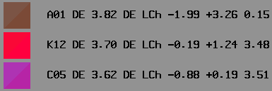
Crop from a patch matching report image. To make it easier to see the difference the patch square has been split diagonally. The reference value is in the top left half, and the profile result in the other.
A few TIFF image files can be dumped:
cm-patch-errors.tif,fm-patch-errors.tif,patch-errors.tif, same as the text files patch matching reports, but showing the actual patches as colored squares.- The patch square is split diagonally, the top left half shows the reference value and the bottom-right what the profile produces.
- The files are 16 bit TIFF in ProPhoto RGB color space (ICC profile is embedded).
- Each file comes in five version with different ordering, first in target order, then in overall DE order, and then ordered by lightness, chroma and hue errors.
- As these are ProPhoto RGB files it's very important that you have display color management enabled, otherwise it will show the wrong colors (typically desaturated).
- If you have super-saturated patches in the target they might clip (rarely in the image itself, but in the color conversion to the screen) which will of course hurt the possibility to accurately visually evaluate the error.
gradient-ref.tif,gradient.tif, generated gradient images for diagnosing profile smoothness.
Plot files
It varies a between commands and parameters used which plot files that are produced, but many will be same, for example if the command processes a target it will produce files related to the target.
Most files have u'v' chromaticity coordinates, and if there's lightness there's CIE Luv / CIE Lab lightness divided by 100. The division by 100 is there to make it about the same scale as u'v'. This is the same 3D space as the DCamProf LUT operates in and is roughly "perceptually uniform", that is moving a certain distance in the diagram makes up a certain color difference. However as the space is linear and lightness is normalized it's not as uniform it could be, especially towards the line of purples which in reality goes towards black and thus hard to differ for the eye.
Here's a list of data files you can find in the report directory after a run:
- Spectra for observer, SSF and illuminant:
cmf-x.dat,cmf-y.dat,cmf-z.dat, the observer's color matching functions.ssf-r.dat,ssf-g.dat,ssf-b.dat, the camera's spectral sensitivity functions.illuminant.datemissive spectrum for the illuminant.illuminant-d50.datemissive spectrum for the standard illuminant D50.
- Common gamuts for u'v' chromaticity diagrams, these are flat but
have three columns to be compatible with 3D plots:
gmt-srgb.dat, sRGB gamut.gmt-adobergb.dat, Adobe RGB gamut.gmt-prophoto.dat, ProPhoto gamut.gmt-pointer.dat, Pointer's gamut.gmt-locus.dat, spectral locus for the chosen observer.
- Gamuts (again u'v' chromaticity only) related to the profile,
either native or imported/generated DCP/ICC.
gmt-cm.dat,gmt-cm2.dat, ColorMatrix gamut. ColorMatrix2 is for DNG profiles only.gmt-fm.dat,gmt-fm2.dat, ForwardMatrix gamut. ForwardMatrix2 is for DNG profiles only.gmt-lm.dat, LUTMatrix gamut.gmt-prof.dat, profile maximum gamut, that is the maximum area the profile will cover for all possible inputs. The profile is coarsely sampled so it may miss some corners.gmt-prof-look.dat, profile maximum gamut, including LookTable (DNG profiles only).
- Files related to the test target, for 3D plots with u'v' and
L/100 except the spectra which are 2D (see also the target files in
the LUT section further down):
target-xyz.dat, XYZ reference values for the patches, usually for the calibration illuminant.target-spectra.dat, reflectance spectra for the patches.target-xyz-<classname>.dat,target-spectra-<classname>.dat, same as above split per target class name.targetd50-*, D50 versions of above. Note that the spectra are the same regardless of illuminant as it's the reflectance spectra.- Live update of spectra and patches during target generation, can
be fun to plot via a gnuplot loop to see spectral generation
progress graphically:
live-patches.datXYZ reference values for the chosen illuminant.live-spectra.datreflectance spectra for the patches.
- Files related to the LUTs, the target files are all relative to
D50 as the LUT works in that space:
nve-lut.dat, native LUT stretching in u'v' difference (addition), plus the L multiplier shown as a 1/10th of the difference from 1.0. The reason for the strange L scale is that the LUT stretching on the L scale should be fairly perceptually equal to the chromaticity stretch. That is any bend on the surface should have equal perceptual effect regardless of axis.nve-lutd.dat, same asnve-lut.datbut the grid is sampled with higher density, useful for zoomed in or high resolution plots.nve-ref.dat, a plain grid showing a LUT with no correction factors, can be used to plot a reference to compare.nve-lutv.dat, vectors that show the difference fromnve-ref.dattonve-lut.dat.hsm-lut.dat,hsm-lutv.dat,hsm-ref.dat, same as thenve-*files, but for the DCP HueSatMap LUT.lkt-lut.dat,lkt-lutv.dat,lkt-ref.dat, same as thenve-*files, but for the DCP LookTable LUT.lkt-lutXX.dat,hsm-lutXX.dat, replace XX with 00 to value divisions-1, shows each value slice from a DCP 3D LUT. Will not be produced for 2.5D LUTs.icc-lut.dat, all points in the ICC 3D LUT plotted in the same space asnve-lut-dat.icc-lutXX.dat, replace XX with 00 to 19, shows slices of the ICC 3D LUT.target-nve-lut.dat, the target patches' XYZ positions after native LUT correction.target-nve-lutvm.dat, vectors showing the difference between matrix-only correction and LUT correction.target-nve-lutve.dat, vectors showing the difference between target reference values (targetd50-xyz.dat) and the profile's final values after LUT, that is the error vectors. For a perfect match these are all zero length.target-nve-lutve2.dat, same as*lutve.dat, but the length of the vector is CIEDE2000, divided by 100 to fit in the u'v' scale.target-nve-lutve3.dat, same as*lutve2.dat, but colors normalized to lightest possible value first, that is what the error would be if the color was light, will significantly increase error for dark colors.target-hsm-lut.dat,target-hsm-lutvm.dat,target-hsm-lutve*.dat, same as thetarget-nve-*files, but for the DCP LUT.target-icc-lut.dat,target-icc-lutve*.dat, same as thetarget-nve-*files, but for the ICC LUT. Note that the*-lutvm.datdoesn't exist for ICC as there is usually no XYZ matrix.target-mtx.dat,target-mtxve*.dat, the target patches' XYZ positions after matrix-only correction, plus the corresponding error vectors.
- Other files
ssf-csep.dat, camera color separation performance.tf-r.dat,tf-g.dat,tf-b.dat, transfer functions for linearizing RGB values.tc.dat,tc-srgb.dat, tone curve in linear and sRGB gamma encoding (both axes).target-ref*,target-match*,target*,target-refm*, target spectra and XYZ plots written by the match-spectra command.glare-curves.dat, glare matching curves from the testchart-ff command (only when glare matching is enabled).glare-match.tif, patch difference chart before and after glare matching.
Example gnuplot scripts
As patch colors are often involved I recommend using gnuplot with a
gray background rather than the default white. If you use the X11
terminal you do this by starting gnuplot with the following
command gnuplot -background gray. All examples here are
adapted for a gray background.
In gnuplot you do 2D plots with the plot command, and 3D
plots with splot. It's often useful to view a 3D plot in 2D
though, and thanks to gnuplot's isometric perspective viewing a 3D plot
straight from above makes it perfectly 2D.
You can rotate a 3D plot using the mouse, and you can zoom
in by right-clicking and drawing a zoom-in-box. Type reset
and replot to return to the original view. It's not a quick
thing to master gnuplot, but with the help of the example scripts here
you should be able to get around and do the tasks necessary for
visualizing DCamProf data.
You can label the axes etc, but I usually make it simple and just
remove all labels with unset key.
Plotting SSF and observer CMF:
  plot \
    'cmf-x.dat' w l lc "pink", \
    'cmf-y.dat' w l lc "greenyellow", \
    'cmf-z.dat' w l lc "cyan", \
    'ssf-r.dat' w l lc "red", \
    'ssf-g.dat' w l lc "green", \
    'ssf-b.dat' w l lc "blue"
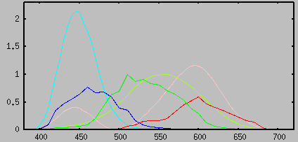
Basic plot for a test target, first the target spectra in 2D:
plot 'target-spectra.dat' w l lc rgb var
The example shows a CC24
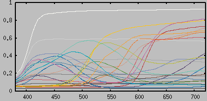
...and then the target patches in 3D:
  set grid
  splot \
   'gmt-locus.dat' w l lw 4 lc rgb var, \
   'gmt-adobergb.dat' w l lc "red", \
   'gmt-pointer.dat' w l lw 2 lc rgb var,\
   'target-xyz.dat' pt 5 lc rgb var
Not shown in the example, but you can also get text labels beside each
patch by adding: 'target-xyz.dat' using 1:2:3:5 with labels offset 2
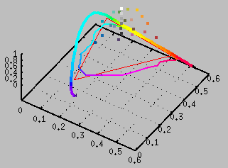
A suitable plot after a make-profile or test-profile
run with a target with relative few patches (such as a CC24):
  splot \
   'nve-lut.dat' w l lc "beige", \
   'gmt-locus.dat' w l lw 4 lc rgb var, \
   'gmt-adobergb.dat' w l lc "red", \
   'gmt-pointer.dat' w l lw 2 lc rgb var,\
   'target-nve-lutvm.dat' w vec lw 2 \
      lc "black", \
   'targetd50-xyz.dat' pt 5 ps 2 \
      lc rgb var
The image shows a zoomed in section, viewed directly from above, so we see a 2D chromaticity diagram with the LUT stretching in the chromaticity dimension. The black LUT vectors are only a little visible as the matrix alone makes a fair match.
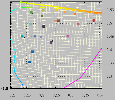
A plot after a test-profile run with a dense target, such as
a locus grid:
  splot \
   'nve-lut.dat' w l lc "beige", \
   'gmt-locus.dat' w l lw 4 lc rgb var, \
   'gmt-adobergb.dat' w l lc "red", \
   'gmt-prophoto.dat' w l lc "blue", \
   'gmt-pointer.dat' w l lw 2 lc rgb var,\
   'target-nve-lutve.dat' w vec lc "black"
Here we only plot the error vectors, the actual color (reference XYZ) is at the start of the arrow and where it ends up after profiling is at the end of the arrow. For a perfect profile on a perfect camera the vector length should thus be zero over the whole field. As we can see in the example to the right errors typically grow large towards the locus, the matrix even moves points outside the human gamut.
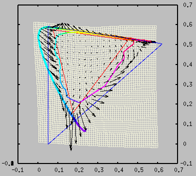
A plot after a test-profile run with a DCP profile:
  splot \
   'hsm-lutv.dat' w vec lc "beige", \
   'gmt-locus.dat' w l lw 4 lc rgb var, \
   'gmt-adobergb.dat' w l lc "red", \
   'gmt-prophoto.dat' w l lc "blue", \
   'gmt-pointer.dat' w l lw 2 lc rgb var,\
   'targetd50-xyz.dat' pt 5 ps 1.2 \
     lc rgb var
Here we plot the DCP HSM LUT as vectors, it can't be plotted like a grid like the native LUT. The vectors show each table position at vector start and their shift in chromaticity and lightness at vector end. Note that a DCP HSM LUT actually changes values through multiplication in linear Prophoto RGB HSV space, that's why the LUT looks like a star fitted in the ProPhoto triangle with high density at the white-point. The lightness axis has been transformed to match the same scale as the native LUT so the LUTs can be compared directly.
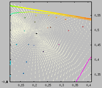
Be careful to watch gnuplot's auto-scaling of axes. The lightness axis in a LUT often gets greatly exaggerated or compressed due to it's not plot at the same scale as chromaticity. Use the set view equal command to turn on/off equal scaling (xyz = equal scaling on all axes, xy = default meaning chromaticity equal and lightness scaled to fit).
  set view equal xyz
  set view equal xy
With equal scale on the L axis a LUT typically looks very flat as L adjustments are generally minor.
More example scripts are found throughout the documentation.
Call for spectral databases and camera SSFs
DCamProf contains some built-in spectral data that has been retrieved from public sources. I'd like to have more. A database with spectral reflectance of human skin is currently the most desired, useful for rendering portrait profiles.
There are reference standard sets such as the ISO TR 16066, but those are not free and cannot be freely redistributed so I can't include that in DCamProf.
If you know of any database you think is useful for inclusion please let me know.
The other aspect is camera SSFs. It's quite complicated and/or costly to measure camera SSFs so most users will not be able to do that and thus have to rely on public sources. If you can provide camera SSFs or have links to sources I have missed please let me know.
Links to camera SSFs
- http://www.cis.rit.edu/~dxl5849/projects/camspec/database.txt
- Part of the work by Dengyu Liu, http://www.cis.rit.edu/~dxl5849/projects/camspec/
- http://www.cvl.iis.u-tokyo.ac.jp/~rei/research/cs/zhao/database.html
- https://spectralestimation.wordpress.com/data/
Links to spectral databases
- http://www.uef.fi/sv/spectral/spectral-database
- Munsell book of colors, spectra from nature, etc.
- http://www.babelcolor.com/main_level/ColorChecker.htm
- Spectral data for the Macbeth colorchecker.
- http://www.cis.rit.edu/research/mcsl2/online/lippmann2000.php
- Spectral data for humans.
- Note: use only allowed for research purposes, therefore data
is not included in DCamProf, but can be parsed with
dcamprof
      txt2ti3 ...
- http://www.reflectance.co.uk/
- "FReD", the Floral Reflectance Database.
Acknowledgments
I'd like to thank those that have made camera SSFs and spectral databases available, without those DCamProf would not have been possible in its current form. Currently DCamProf has spectral databases from University of Eastern Finland and BabelColor, see the section with links to spectral databases for references.
I also would like to thank all early adopters for testing the software and providing valuable feedback.
Thanks to Mike Hutt for the Nelder-Mead simplex implementation which is used in DCamProf for solving various multi-variable complex optimization problems. I also want to thank Jarno Elonen for publishing a thin plate spline implementation which served as base for the DCamProf TPS used for getting a smooth LUT.
The copyright for the TPS source is required to be repeated in the documentation, so here it is:
  Copyright (C) 2003, 2004 by Jarno Elonen

  Permission to use, copy, modify, distribute and sell this
  software and its documentation for any purpose is hereby
  granted without fee, provided that the above copyright
  notice appear in all copies and that both that copyright
  notice and this permission notice appear in supporting
  documentation. The authors make no representations about
  the suitability of this software for any purpose. It is
  provided "as is" without express or implied warranty.
Copyright © 2015 – 2018 — Anders Torger.