|
01-01-13
|
|
|

Software Equaliser and Tools for High Resolution Digital
Audio
Keywords:
equaliser, filter, room equalisation, room correction, high fidelity digital
audio, real-time software, WFIR (Warped Finite Impulse Response), MLS (Maximum Length Sequence),
FHT (Fast Hadamard Transform), FFT (Fast Fourier Transform), impulse
response measurements, GSL (GNU Scientific Library), ALSA (Advanced
Linux Sound Architecture), GNU General Public
License, open source.
|
News
01-01-13
This project is now no longer being developed. Large parts of the code
will probably be reused in future projects though.
00-10-15
Added a note at the top of this page, indicating what is worked on.
00-10-01
Added a FIR filter designer.
00-09-16
Some bugfixes, new impulse response
post-processing program.
00-08-13
Optimised/bug-fixed buffering in nwfiir.
00-06-17
Updated ALSA pre-0.6 support in nwfiir.
00-06-11
FIR filter engine in nwfiir is now usable.
00-04-17
Strongly improved realtime performance of nwfiir thanks to a
new buffering system.
00-03-18
ALSA support implemented
in nwfiir.
00-03-12
Digi96 driver available (I
wrote it). Sample format flexibility added to the tools. Preliminary
FIR filter engine in nwfiir, not for practical use yet though.
00-01-30
Further development of the suite is currently on ice. I'm waiting
for Linux drivers to the RME Digi96 digital I/O.
99-12-12
Have received measurement equipment, and performed room equalisation
successfully with promising results. New release with a few bugfixes.
99-12-05
Verified that the package is compatible with GSL 0.5.
Still no microphone nor A/D converter.
99-11-28
I have unfortunately not yet got a microphone and A/D converter as I
had planned. It will be at least one more week before I can test the
room equalisation system in practice.
99-11-21
Fixed a couple of bugs in nwfiir. Released mls2imp, a program for
extracting the impulse response from an MLS response. Started
reworking this page.
99-11-17
Simplified mlsgen, and removed an embarrassing bug from it. I still would
not recommend using it before I have tested it in practice
though.
99-11-14
Included a power response pre-processor to be used prior to filter
design on measured power responses.
99-11-13
Fixed permission bug for shared memory in nwfiir.
99-11-07
Extended nwfiir to handle other warp factors than 127/128. Also, the
threaded implementation has been dropped in favour of a solution using
fork and shared memory.
99-11-02
A fatal bug in the Maximum Length Sequence generator has been
corrected. Now it should (hopefully) generate correct MLS sequences.
99-10-31
A Maximum Length Sequence generator is now included in the
package. Getting closer to providing a complete room equalisation system.
99-10-27
Compability issues with GNU Scientific Library 0.4.1 resolved.
99-10-26
Added automatic gain adjustment in the WFIR filter design program.
99-10-24
Initial release.
|
|
Note: the text on this web page is largely out of
date (and contains some factual errors). The nwfiir program suite is no
longer being developed, thus no further updates can be
expected. However, if you are interested in nwfiir, it is likely
that you also are interested in
BruteFIR.
Table of
Contents
- What is this stuff?
- What is room equalisation?
- Digital equalisation -- practical issues
- How to make your HiFi-system sound better in eight not-so-simple steps
- Tips & tricks
- Download!
- Acknowledgement
- References
What is this
stuff?
Nwfiir audio tools is a free suite of console programs for your Unix
machine (Linux in particular) to process high resolution digital audio. The suite's core
program is nwfiir, which is a real-time digital equaliser. The
name is a combination of the abbrevations FIR, IIR, WFIR and WIIR, that is four types of filters,
Finite Impulse Response, Infinite Impulse Response and their warped
counterparts. Currently only FIR and WFIR have been implemented. The
leading n stands for that it is capable of an arbitrary amount
of channels. Below is the current list of the complete set of tools included in the
suite:
 |
nwfiir
-- Equaliser designed for real-time operation. The task for an audio equaliser is to
amplify frequencies in sound according to a given power response
(often referred to as magnitude spectrum or frequency response). One
could for example produce an extra bass boost by amplifying
frequencies around 50 Hz. Of course, this can be done with an ordinary
analogue equaliser, and indeed, bass and treble control exist on many
HiFi amplifiers. The advantage of this digital equaliser is that it
has a large amount of bands, so the power response can be precisely
tuned over the entire audible range. It takes advantage of machines
having more than one processor.
|
|
wfird
-- WFIR filter designer. This program is used to
calculate filter coefficients for a WFIR filter to fit a given power
response. The coefficients are then fed into nwfiir, to produce the
complete working equaliser.
|
|
mlsgen
-- MLS (Maximum Length Sequence) signal generator. This program is
used to generate a periodic pseudo-random sequence that for example
can be used as an excitation signal for a speaker to indirectly measure its
impulse response. How it sounds? Like an evenly spread noise, so it is
easier to endure than other common excitation signals, like swept sine.
|
|
mls2imp
-- MLS to impulse response converter. When mlsgen has been used to
excite a speaker and its sound has been recorded, that recorded signal
is fed into this program to reveal the impulse response. From the
impulse response the program can also calculate the power and phase response.
|
|
mspreproc
-- Magnitude spectrum pre-processor. This is used to smooth a measured
power response (magnitude spectrum) before it is used for filter
design, in wfird for example. The current implementation is a hack, it
works but I'm not very proud of it.
|
So, what should all these programs be used for then? Well, for anything
you like. However, I programmed this suite for a single purpose, namely to
improve the sound of my HiFi-system with room equalisation. Perhaps
you also want to improve the sound of your Hifi-system,
or just play around with the equaliser on your MP3s or something,
but you don't understand all this impulse response stuff I'm writing
about. Well, you do not need to understand it either, I don't. I have
written step-by-step guides of how to use the software.
What is room
equalisation?
The goal of room equalisation is to
have a desired power response in the listening position. The desired response is most
often the flat one, that is when all frequencies in the audible range,
from 20 - 20000 Hz, are equally amplified. You may own very expensive speakers and
amplifiers and so on, that will produce a flat power response, but
only if it is placed in an anechoic lab environment. The room have a
profound impact on the sound. To minimise the problems, one can measure the power response in
the listening position with a microphone, and with help of that put in a
precisely tuned equaliser that minimises the room's negative impact on the
sound. Commercial systems exist for this (Roister,
Tact Audio), however they
are still very, very expensive. The software presented here is a
a full room equalisation system, apart from the hardware which you may well
own already anyway.
|
|
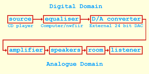
Figure 1. Room equalisation diagram showing a setup using the
nwfiir software.
|
Figure 1 shows a typical setup for room equalisation using nwfiir
as equaliser. Note that all calculation is done in the digital domain,
not until the D/A converter (DAC) the signal gets analogue. The
difference between this and an ordinary setup without the equaliser is
that the DAC is usually integrated into the CD player, instead of
having an external.
Many audiophiles believe that room equalisation is used to improve sound in
low quality Hifi-systems. This is not true, even the most expensive
systems will benefit from it, then mostly in the bass
range. It is also a common belief that an acoustically treated room
(drapes, diffusors, bass traps etc.) does not need room equalisation.
This is also not true, acoustic treatment is simply not precise
enough. This does not mean that acoustic treatment is meaningless, it
is very useful in correcting problems room equalisation (in full) cannot, that
is reflection-oriented problems.
Digital equalisation -- practical issues
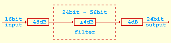
When a digital filter is deployed to equalise audio, two important issues must
be considered. 1) output sample range must be reduced to avoid
overflow and 2) output should be of higher resolution than input.
Equalisation normally means that some frequencies are amplified.
If we amplify the signal, it means that samples will be multiplied
with some value larger than one. This means that there is a risk for
overflow. If the original sample is the maximum value (+32767 and
-32768 for 16 bit) we cannot amplify it without overflow, which yeilds
a seemingly random value. Therefore we must lower the signal power
with about as much as the filter will amplify to be on the safe
side. It is possible to gamble a bit, for example if the digital sound
is not expected to use the full range (common in classical music
recordings). We want to lower as little as possible, since lowering
the signal power means that we get closer to the noise floor both in
the digital and analogue domain.
When filtering, there will also be requantisation error. If we scale
the sample value +1452 up with three percent, we get +1495.56, but
since the samples are integers, it will be rounded to +1496. This
procedure is called requantisation. To make things worse, the
original sample has been rounded once already, from an analouge source,
or a digital with higher resolution. To reduce the effects of
requantisation error, it is necessary to have higher resolution on the
output of the filter than on the input. The usual way would be 16 bit
input (from CD) and 24 bit output.
Internally, most filters make some kind of accumulation of sample
values multiplied with some constants. To avoid overflow while keeping
high resolution, an accumulation register of at least 56 bits is
needed. This is available on modern DSPs (Digital Signal Processors),
however when implemented on an ordinary 32 bit processor like the
Intel Pentium, two 32 bit registers joined together to 64 bits are used.
(Stuff about redithering and floating point filters should be added
here)
|
|
Figure 2. Typical sample scaling of a high quality
digital audio filter working as an equaliser.
|
How to make your
HiFi-system sound better in eight not-so-simple steps
Here I will give a step-by-step guide of how to install and configure
this room equalisation system for your HiFi-system. Although you may
not want to use the suite for room equalisation, it may be worth
reading some of the steps, since they contain instructions of how to
use the programs. The steps are:
- Gather hardware -- describes what hardware is required.
- Setup the hardware -- tips on how to arrange the hardware in a
flexible way.
- Measure the MLS response -- how to indirectly measure the impulse
response in the listening position.
- Get the power response -- how to extract the power and impulse
response from the MLS measurement.
- Pre-process the power response -- how to pre-process the measured
power response before it is fed into the filter designer.
- Generate filter coefficients -- how to use the filter designer.
- Test equalisation and do eventual adjustments.
- Enjoy! -- conclusion.
 |
Gather hardware
This is probably the hardest step, because this is the time to realise
that you perhaps must shell out some money. This is what you will need:
- A room.
- A HiFi-system with digital or analogue input to receive sound from the computer.
- Music good enough to make the effort equalising worth it.
- Digital or analogue output on a fast computer running a flavour of
Unix, (currently Linux is the only flavour that is fully supported) for
example the free Debian GNU/Linux.
- Digital or analogue output from the HiFi-system, and corresponding
input on the computer, or alternatively a CD-ROM drive in the computer with good CD-rip performance.
- A measurement microphone with additional equipment to get the measured signal into the computer in digital form.
Although it is possible to use analogue connections between the
HiFi-system and the computer, its is not recommend. You should at
least have digital output from the Hifi-system and corresponding digital input on
the computer, or use the computer's own CD-ROM drive to play the CDs. Then you can use a sound card's DAC to produce an
analogue signal to send to the amplifier, but it is generally not a good idea,
since the quality of the DAC is likely not good. Better is to
have digital output from the computer and an external HiFi DAC
connected to the amplifier with short high quality signal cables.
To keep a fully digital chain as long as possible I use Musical Fidelity's
DAC X-24K, and RME-Audio's
digital I/O board DIGI96. When you run Linux, transferring digital
data between the I/O board and the program can be a
problem, since many of these boards lack drivers. A driver for the DIGI96
exists in ALSA, which is a
sound card driver architecture for Linux. It aims to replace the
outdated (and commercial) OSS. The choice of I/O board is important, not just
because of the drivers, but also that some of these so called digital
sound cards alters the signal (amplification, equalising and other
mumbo-jumbo may be performed by an on-board low quality signal processor).
If you are going to use both the input and output on a single sound
card (or digital I/O) it is important that it is
capable of full duplex operation, and can handle different formats at the same time (that
is for example 16 bit 44.1 kHz on the input and 24 bit 44.1 kHz on the
output). For best sound quality the DAC should be able to handle 24 bit digital
audio signals. Also, it may be a good idea to make sure that the DAC
reclocks the signal (not all do unfortunately), or else the sound may
be degraded by jitter in the transfer process. It's much more wise to
buy a well designed reclocking DAC than expensive digital transfer cables.
When it comes to the microphone, you probably should borrow or rent
it. You will only need it for a brief time, and buying an own is
quite expensive. A good microphone should have an error less than +/- 1 dB in
the range 20 - 10000 Hz, but between 10000 - 20000 Hz one can allow a
larger error like +/- 2 dB. Apart from the microphone you will
need a microphone pre-amplifier and an ADC (Analouge to Digital
Converter). The ADC could be on a sound card, or in a
DAT-recorder for example. Sometimes the the ADC is equipped with an
amplifier on the input so you do not need a microphone pre-amplifier.
You will not need to get the sound into the
computer in real-time.
You may wonder how fast a fast computer is. I use a dual Pentium II
running at 266 MHz. The equaliser makes use of both processors. It is
enough with some marigin to get good equalisation. You could use a slower machine,
but then you will have to sacrifice equalisation resolution. A
single processor machine of 400 MHz or more should be fine. Some code
is written in highly optimised x86 assembler, which means that the processor will need
to be a Intel processor or compatible. Or, you just write your own
assembler code for your processor and send it to me for inclusion in the
software package.
Let us conclude with a listing of the hardware I use for my room equalisation:
- Dual Pentium II 266 MHz running Debian GNU/Linux.
- RME Audio DIGI96 digital I/O board.
- Musical Fidelity X-24K, 24 bit 44.1 - 96 kHz external D/A
converter.
- RME Audio ADI-1, 20 bit 32 - 48 kHz external A/D D/A converter. Used
for measurements.
- Clio Microphone Lite, +/- 1 dB 20 Hz - 10 kHz, +/- 2 dB 10 - 20 kHz.
- Cable to feed power to the microphone with a 9V battery.
Again, you should not buy the measuring equipment if you're not
very interested in doing measurements. If you decide to do it, you
could buy the ADI-1 and use it both for measuring and as external HiFi
DAC. I have not tested how it sounds though, but it is certainly better than most consumer sound
cards. For the measurement task the ADI-1 is used for here, it is
probably a bit better than it need to be. An ordinary cheap sound card would probably
do, however the frequency response of the low frequencies (below 40
Hz) tend to be poor, I've heard. The quality of the DAC you choose should of course mirror the quality of
your HiFi-system. This is mine (the relevant parts):
- Electrocompaniet ECI-1, integrated amplifier.
- B&W CDM7, three-way speakers. Used as front channels.
- B&W DM 601 S2, two-way speakers. Used as rear channels.
- A too small listening room (3.5 times 4.5 meters).
The CD player should be the cheapest possible that provides digital
output, or you could, as mentioned earlier, use your computer's CD-ROM
drive and a good ripper program like cdparanoia. If you use an
ordinary HiFi CD player you should know that even the cheapest players
read all bits from a normal CD correctly after ECC (ok, perhaps the
first few milliseconds when starting to read get a bit messed up, they
get that on my CD player),
no matter what "HiFi experts" say. A lot of expensive CD
players sell on the myth that it is hard to get the samples from the
CD in a correct way. Keep in mind that less than 60% of all bits on a
CD is effective samples, almost all the rest are for error correction.
The rear channels I have connected is a special arrangement that enhances room
acoustics on the recordings, but that is another story. They lay about
12 dB below the front speakers so they can be ignored in the
measurements.
|
 |
Set up the
hardware
First you should review your speaker placement, and room
environment. It should be set up as good as possible before
equalisation. Although equalisation probably will improve the sound
of poorly placed speakers, correctly placed equalised speakers will
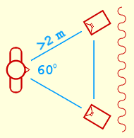
sound even better. Since phase will not be corrected, it is still very
important to have the speakers at equal distance from the listening
position. The equilateral triangle placement shown in figure 3 is a
good reference. Placing heavy drapes on the wall behind the speakers
to absorb reflections is a good idea, as well as having diffusing
material on the opposite wall. This is the Live-End Dead-End layout
common in professional sound studios. However, I shall not get into
all details of speaker placement here, since you probably already know
them.
|
|
Figure 3. Basic listening room layout with drapes.
|
Now you should decide what you want to have as principal sound
source. Normally that would be your CD-player in the listening
room. But you could also use your computer for playing MP3, or playing
straight from its CD-ROM drive. I will assume that you will use the
HiFi-system's CD-player, that is also what I do, most of the time. Many CD-players have
two digital outputs, one coaxial and one optical. They send the signal
on both outputs at the same time, so you can use both of them if you
like. That way you can lead one output to the computer, and one
directly to the DAC, so you can play CDs without having the computer involved.
A problem with computers is that they are noisy. You will probably not
want to have your computer in the listening room. Therefore you will
need long digital transmission cables. But that is no problem, you can
have up to 10 meters (probably even longer, but I have not tested).
It is a good idea to make them for yourself, do
not buy them in an HiFi store, since they will try to fool you with
jitter bullshit and make you buy extremely expensive cables. Jitter is
only a real problem with DACs that lack reclocking circuitury and/or
are poorly designed. Sure, you may have such a DAC, but then it is
much better to put your money into a well designed DAC than expensive
cables. The computer just need the bits in correct order, so it is
insensitive to normal amounts of jitter.
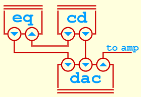
So, now we have a digital transmission cable running from the
CD-player in the listening room, to the digital input in the computer
(which probably is located in another room). Also, we have a cable
from the digital output on the computer to one of the digital inputs
on the DAC. Additionally, to be able to bypass the computer, we use
the second digital output from the CD-player and connect it directly
to another input on the DAC. The DAC's anolouge output is of course
connected to the HiFi amplifier. Below is a schematic picture showing
the setup. Eq is the equaliser, that is the computer.
|
|
Figure 4. Example of how to connect CD, DAC and equaliser.
|
Lastly, a note about equalisers that may already exist in your HiFi system. You
may have treble and bass control on your amplifier, or a multi-band
equaliser. All those should be set in neutral position before proceeding.
|
 |
Measure the MLS response in
the listening position
To measure the MLS response we need an MLS excitation signal to the
speakers. This is given by mlsgen. The resulting sound is then
measured by the measurement microphone in the listening
position. In some way you must get the measured signal into the
computer. How this is done depends on what microphone setup
you have. Perhaps you record with a DAT recorder first, and use the
digital output from it to get the signal into the computer later. This
is possible since there is no need to
get the sound into the computer in real-time. Another example is to
use a recording system under another operating system, such as
Microsoft Windows, and save the recorded sound to a .wav-file
for later use. Actually, if you have other software that can measure
power response and export is as a text file, you could use that
instead of the audio tools presented here. However, I assume that you
will use my programs. So, you have to know how to use mlsgen.
The purpose of mlsgen is to generate Maximum Length Sequences. An MLS
is a carefully calculated noise signal used to indirectly measure a
system's impulse response in a background noise robust way. If you are
interested in the theory behind it you should be able to find it at
MLSSA's (pronounced
"Melissa") website. MLSSA is a commercial MLS measuring
system. However, now let us concentrate on the free mlsgen, and look
at its parameters by running it without any.
M L S G E N -- a Maximum Length Sequence Generator         Experimental version
==================================================            (c) Anders Torger
                                                                      Mars 2000

Usage: mlsgen [-it] [-a <amplitude>] [-b <output format>]
        [-c <n channels>[,<output ch>,...]] [-p <n samples>]
        [-r <n times>] [-s <tap set index>] <order>

 -i use IRS (Inverse Repeated Sequence)
 -t print sequence as text (once), values will be -1 and 1. Other optional
    parameters will be ignored (except -i)
 -a <amplitude> amplitude for the MLS values, from 0.0 - 1.0. Default: 0.5
 -b <output format>, <bits><s(igned)/u(nsigned)><bytes><l(ittle)/b(ig) endian>
    <left shift>. Default: 16s2l0
 -c <n channels>[,<output ch>,...] number of channels and in which channel(s)
    to play. Default: 1,1
 -p <n samples> width of pulse in samples. Default: 1
 -r <n times> number of times to play the output sequence. A value less than 1
    means infinite number of times. Default: 1
 -s <tap set index> choose tap set, to vary an MLS of the same order.
    Default: 0
The most important parameter is the one which chooses the length of
the test signal, that is the order of the MLS. It is important that
the impulse response to be measured contain all its significant energy
within the duration of the MLS. This length can only be roughly
approximated, but that is no problem since we need not be exact. The
order 16 - 18 should be enough for all normal listening rooms, at a
sampling rate of 44100 Hz. The length of the MLS is 2^<order>-1, for
order 16 that becomes 2^16-1 = 65535 samples, which is about one and a
half second.
You should measure one channel at a time, that is play and record the
MLS in one channel at at time. Below is a typical command line playing
the MLS through the left channel in a stereo system:
mlsgen -c 2,1 -r 2 18 ¦ aplay -m
I choose to play two channels, with sound
in the first, that is the left channel, with the parameter -c
2,1. Then I instruct mlsgen to play the signal twice, with
-r 2. A fine thing with MLS
measurement is that timing does not matter. As long
we record when MLS noise coming out from the speakers it is
ok. Therefore I let the signal play twice, so I easily can record at
least one length of the signal. The player in this case is aplay,
which is the player included with ALSA. I will use that throughout the examples.
Be careful so you don't put to much power into the speakers when
playing the MLS. The noise should be around normal listening levels,
perhaps a bit above to reduce effects of background noise. If you stress
your speakers with too much power, not only can they be
damaged, the MLS measurement may also be distorted. It is also
important that the sound level is not changed during recording, since
it will distort the measurement.
When you have tested that mlsgen works as you wish, it is time to set up
the microphone. It should be mounted in the listening position, at
listener's head height. Some say it should be pointed in a way
that the direct sound from the measured speaker produce a flat
response in the microphone. For example if the microphone produces a
flat response when sound is coming straight to it, it should be pointed
straight at the speaker to be measured. Others say that the microphone
should be pointed at the ceiling. I have tested both, and it did not
induce any significant difference. Under the measurements presented
here, I kept the microphone pointing at the ceiling.
Note that it is not necessary to measure absolute levels of sound,
that is you will only need to measure sound pressure with a common
reference for all measured channels. So if you don't calibrate your
equipment to a certain reference, it does no matter as long as all
channels are measured with the same setting.
After you have set up the microphone, you just record noise from each
channel and store the recorded data on hard disk. Although the measurement method is quite noise
robust, try to have as little background noise as possible.
|
 |
Get the power response
Ok, so now you have measured the MLS response for each channel.
Now it is time to do some number crunching to get the power response for
each channel as heard in the listening position. A
power response can be calculated from the impulse response with the
help of the Fast Fourier Transform (FFT). The mls2imp program
calculates an impulse response from an MLS response, and can from that
apply the FFT to get the power or phase response. Let us see the
output from the program when it is not given any parameters.
M L S 2 I M P -- MLS Response Processing Program           Experimental version
================================================              (c) Anders Torger
 Uses FHT and FFT to find impulse/power response                      Mars 2000

Usage: ./mls2imp [-himruwx] [-b <input format>]
       [-c <n channels>,<target channel>] [-f <input filename>]
       [-o <n seconds>] [-p <n samples>] [-q <sampling frequency>]
       [-s <tap set index>] <MLS order>

 -h get power response.
 -i get minimum phase response.
 -m get power response in decibel.
 -r output as text in hexadecimal memory dump format.
 -w get phase response.
 -x get excess phase response.
 -b <output format>, <bits><s(igned)/u(nsigned)><bytes><l(ittle)/b(ig) endian>
    <left shift>. Default: 16s2l0
 -c <n channels>,<target channel> number of interleaved channels and which of
    them that holds the MLS response to be processed. Default: 1,1
 -f <input filename> file to read data from. Default: read from stdin
 -o <n seconds> number of seconds to ignore in the beginning. Default: 0
 -p <n samples> width of pulse in samples of original MLS. Default: 1
 -q <sampling frequency> sampling frequency in Hz of input. Default: 44100
 -s <tap set index> must be same tap set as the original MLS. Default: 0
It has a lot of parameters, but it is most often only necessary to use
a few of them. Let us assume that you have recorded 10 seconds of two
channels playing MLS noise of the 18th order
in 16 bit 44100 Hz and saved the sound to the files ch1mls.dat and
ch2mls.dat. Mls2imp is only interested
in the raw samples as input, any sound format headers would only mess
things up. Therefore if you have recorded for example
.wav-files, you must remove the headers. In the
.wav-file case the header is 44 bytes, and the rest is the
raw samples saved in little endian byte order. To remove the leading
44 bytes you can for instance use the tail command. Now, this
is the way you could run mls2imp:
mls2imp -m -c 2,1 -f ch1mls.dat 18 > ch1pow.dat
With -m the program is instructed to output the power
response in decibel, as calculated from the impulse response. Although
the microphone is mono, most recordings are done in stereo. With the
-c 2,1 parameter, the program will read the input as two
channels, but only pick data from channel 1, where hopefully the
microphone recording is. The
output stored in ch1pow.dat will contain two colums with
numbers, the first frequencies, the second magnitude in decibel. This
file can directly be plotted in gnuplot (or any other good plotting program).
Below you see how the plot of the magnitude response looks like for my
left channel in my listening room.
|
|
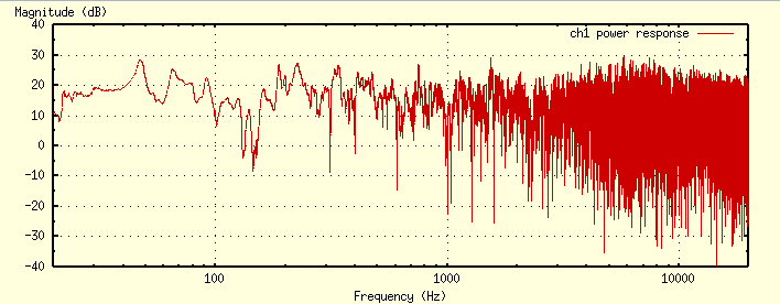
Figure 5. The power response of the left channel as measured in the
listening position.
|
If you think your measurement is a bit strange in some way, you can try to use the
-o parameter to use another set of samples from the recorded
data.
As you can see, my power response is not at all flat, as I would
like it to be. The trick is to design a filter that has a power
response equal to the inverted power response seen in the figure. This
way when the sound is filtered through it and played through the
speakers in the room, the resulting, equalised, power response will be flat. So,
let us get on with the next step.
|
 |
Pre-process the power
response
The filter we are going to create for the equalisation, will not be
able to adapt to all details in the measured power response. But that
is not a problem, since we would not want it to, since the measured response of course contains
measurement errors. Also, if it was possible to correct the response
perfectly, we would need to clamp our heads in the listening position,
since moving the head a few centimeters would ruin the high frequency
equalisation.
There is no meaning to adapt to features that
simply are measurement noise. Therefore we want to smooth the
power response.
We are more interested of details in the bass range than in high
frequencies. There are two reasons for this, the first is that there
are usually more problems in the bass range, induced by room modes,
and the second is that the human ear is in this range more sensitive
to narrow band phenomena.
The ear is also more sensitive to peaks in the power response
than dips. This is good, because we do not want to make a filter that
needs to amplify much (why is explained in step 7). The tool used for
pre-processing the measured power response is mspreproc. Running it
without parameters brings up this screen:
M S P R E P R O C  -- a Magnitude Spectrum Pre-processor   Experimental version
========================================================      (c) Anders Torger
      Designed for Room Equalisation applications                 December 1999

Usage: mspreproc [-iorst] [-b <low>,<high>] [-f <input filename>]
       [-g <max gain] [-m <interpolation method>,[resolution]]
       [-v <offset>] [-w <low>,<high>] <smoothing method> [<option(s)>]

 -i input values are in decibel
 -o output in decibel
 -r output values in raw hexadecimal format.
 -s output smoothed magnitude spectrum, instead of the target spectrum.
 -t input is the actual target spectrum, and not the measured room response.
 -b <low>,<high> output spectrum bounds in Hz. Default: 0,22050
 -f <input filename> file to read data from. Default: input read from stdin
 -g <max gain> maximum gain in decibel for correcting dips. Negative value
    means infinity. Default: 3
 -m <interpolation method>,[output length] choose interpolation method, SPLINE,
    LINEAR or NONE. Resolution is in Hz. Default: SPLINE,16384
 -v <offset> offset input spectrum with <offset> dB. Default: 0
 -w <low>,<high> output spectrum interesting bandwidth in Hz. Default: 40,16000

 <smoothing method> [<option(s)>] choose smoothing method from one of the
 methods descriped below:
   SPLIT [split frequency] [low octave fraction] [high octave fraction]
     dual octave bandwidths with a split frequency. Default options are
     "200 1/16 1/3", which means below 200 Hz 1/16 octave smoothing is
     performed, above 1/3.
   WARP [warp factor] [sampling frequency] [n taps] [maximum resolution]
     use bandwidths corresponding (approximately) to the resolution of a warped
     filter. Default options are "127/128 44100 200 1/16".
Magnitude spectrum is just another name of power response. Magnitude
spectrum sounds cooler, so I picked that for this program.
In this step we are after the input to the filter
designer. That is the power response of the filter, which will be the
inverted measured power response with smoothing. It may take quite a
few runs of mspreproc with different parameters before you are
satisfied with the result. This is an example of a good starting point
mspreproc -i -o -s -g -1 -w 20,16000 -f ch1pow.dat split > ch1target_plot.dat
The program assumes that the input data is a measured power response,
and that the output should be based on the inverted
response (also called target spectrum in this context). Therefore you need not to
specify any options for the inversion. However at first it is easier to
create a smoothing of the measured power response instead of a target
spectrum, therefore I have set the -s parameter in the example. The frequency bounds of the
output is kept to the default, that is 0 - 22050 Hz. The the
default maximum gain, which is 3 dB, is removed. This means that the output
spectrum will not at any point have higher than 3 dB
amplification (assuming nothing bad happens during interpolation). The interpolation method, that is the method to extend averaged
frequency points to a full range of equidistant points, is left to the
default. This is spline interpolation, which is not entirely stable,
so in some rare cases the output is not good, you have to check this
by plotting the data. It is not interesting to do equalisation in areas where the
speaker cannot deliver sound, or there is a risk to damage it if we
amplify too much. Often it is not wise to equalise below around 40 Hz,
but if you have good speakers that can handle even low bass, you
should equalise that too. In the highest frequencies the
filter we are going to use will not have high resolution, and probably
the microphone used during measurement has poorer precision. This
combined with that there is little information in the highest
frequencies and that the wave length is very short
making equalisation unfeasible the upper limit is set to 16
kHz. The default range is 40 - 16000 Hz, but since I have speakers
that can handle low bass, I extend it down to 20 Hz, with the
parameter -w 20,16000. As smoothing method the
"split" method is chosen, with the default settings. Narrow
bands are then used in the low frequencies and wider in the high.
Smoothing with this program is not an exact science, therefore it is
important to plot the output and compare with the input and see if the
important features are kept, while non-important are removed. You must
try with different parameters until you have got a good smoothing of
the power response, thereafter you remove the -s parameter to
get the inversion, that is the target spectrum. Then you will probably
also need the -v to adjust the offset of the target spectrum
so it starts and ends close to 0 dB at the bandwidth edges
(20 - 16000 in this example) if it is not possible to get to zero at
both ends, you should give higher priority to the low frequency, in
this case 20 Hz. Additionally, you should specify the maximum gain
with the -g parameter. The gain should be small, the default
is 3 dB which is a good value. As mentioned before, it is more
important to lower the peaks than filling up the dips. So if setting
a low maximum gain will make your dips not being entirely filled, it is
no problem. It is important to keep the offset (-v)
equal for all channels, to get the same sound volume from them in the end.
Now, let us see some figures from my equalisation:
|
|
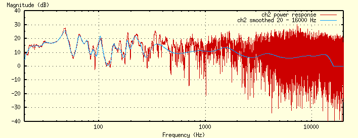
Figure 6. The power response of the right channel as measured in the
listening position, together with a smoothed rendering.
|
In figure 6 the right channel is seen, and a smoothed rendering of it
that I made by running mspreproc with the following parameters:
mspreproc -i -o -s -g -1 -w 20,16000 -f ch2pow.dat \
split 300 1/16 1/3 > ch2smooth.dat
Then I removed the -s parameter, set the maximum gain to the
default, and searched for a suitable offset. The resulting target
spectrums are seen in figure 7 below.
|
|
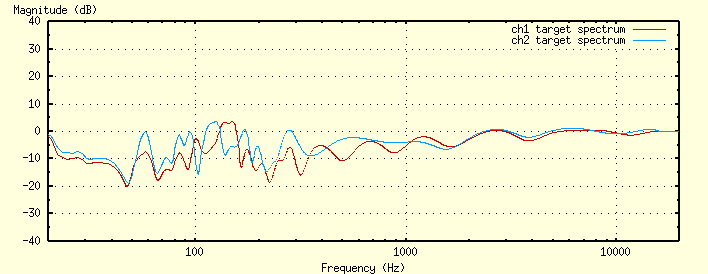
Figure 7. The target spectrums for channel 1 and 2.
|
The command-lines for these target spectrums were:
mspreproc -i -o -w 20,16000 -v -7 -f ch1_pow.dat \
split 300 1/16 1/3 > ch1target.dat

mspreproc -i -o -w 20,16000 -v -7 -f ch2_pow.dat \
split 300 1/16 1/3 > ch2target.dat
When this procedure is completed for all channels, it is time to run
the filter design software. Let us get on with the next step.
|
 |
Generate filter coefficients
Now it is time to generate filter coefficients from the pre-processed
power response. This is done with wfird, since we want to generate
coefficients for a WFIR filter. The output from wfird can then be used
by nwfiir. Wfird takes a file as input, which
should contain two columns, the first should contain frequency numbers
in Hz, the second amplification, optionally in dB. This is what are
in the files ch1target.dat and ch2target.dat
generated in the preceeding step. The filter coefficients should be
generated for each channel.
If wfird is run without parameters, this is its output:
W F I R D -- real valued wfir design                       Experimental version
====================================                          (c) Anders Torger
                                                                      Mars 2000

Usage: wfird [-ior] [-d <output option>] [-f <fft size>] [-g <gain in dB>]
       [-s <sample frequency>] [-w <warp factor>]
       <target power response file> <number of taps>

 -i power response input is in decibel
 -o output in decibel
 -r output memory images of the values rather than human readable form
 -d <output option> selects what to output:
    COEFFS    -- filter coefficients (default)
    TARGET    -- target response (interpolated)
    FILTER    -- filter response
    PHASE     -- filter phase response
    WTARGET   -- warped target response
    WFILTER   -- warped filter response
    ERROR     -- difference between target and filter response
    ALL <dir> -- output all of the above to the directory given.
                 Filenames are coeffs.dat, target.dat, etc.
 -f <fft size> Fast Fourier Transform working set size. Indirectly specifies
    the frequency resolution which is <sample frequency> / <fft size>.
    <fft size> must be a power of two. Default: 32768
 -g <gain in dB> filter gain in decibel. Default: auto gain
 -s <sample frequency> default value: 44100
 -w <warp factor> default value: 0.9921875 (which is 127/128)
I would recommend to run the program like this as a first try:
wfird -i -o -d all . -w 0.984375 ch1target.dat 200
In this example, the number of taps is 200. The number of taps decides
the resolution of the filter, the more taps, the better resolution. Of
course, the more taps, the more processor power will be needed by
nwfiir. 200 taps should be enough in most cases. A rough formula of how
many taps possible for real-time operation in 44100 Hz is the
computer's MHz divided by the number of channels. We can start off
with a rough guess and do fine adjustments later.
The warp factor decides how the filter's bands should be distributed
over the frequency range. We want a warp factor close to one, since it
will lead to small bands in the bass range, and wider bands in the
higher frequencies. However, the standard value (127/128) is probably
a bit too extreme, so I recommend choosing 63/64 instead, which is
0.984375. Nwfiir supports only a fixed set of warp factors, from
1/2, 3/4, 7/8 to 255/256, so you much use one of them.
The parameter -d all . instructs the program to write various
data files that can be plotted in for instance gnuplot. The file
filter.dat is the response of the filter, and
target.dat is the interpolated target, that is
ch1target.dat. The file error.dat contains the
difference between the filter response and the target response.

|
|
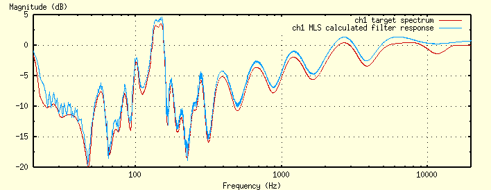
Figure 8. The target and filter response of channel 1.
|
In figure 8, the target spectrum and the filter response of channel 1
is plotted. As you can see, the precision is very good. The resolution
gets lower with higher frequencies, and we can see that it cannot
adapt fully above 10 kHz. If you are not satisified with your result,
you can try to increase the number of taps, and/or change the number
of taps to see if you can get a better result. In rare cases the output
from wfird is a bunch of undefined values, I am not sure what causes
this problem. However, if that happens, try changing the warp factor
very very little, from 0.984375 to 0.98437500001 for example. This
makes the problem go away.
When you are satisfied,
you should generate the filter coefficients in raw format, like this:
wfird -i -r -w 0.984375 ch1target.dat 200 > ch1coeffs.dat
wfird -i -r -w 0.984375 ch2target.dat 200 > ch2coeffs.dat
Raw format means that instead of human readable numbers, the output
values will be raw memory images of the floating point numbers. This
way full precision is preserved. The -r parameter is
available in mspreproc and mls2imp too, but it is a lot less important
to be precise with those.
When you have generated the coefficients, you are at last ready to run
the filter and see, well, hear, your first results of room equalisation.
|
 |
Test equalisation and do
eventual adjustments
Let us see the parameters of nwfiir, as always by running it without
any:
N - W F I I R -- a real-time filter engine for audio       Experimental version
====================================================          (c) Anders Torger
   Designed for High-Fidelity audio applications                      Mars 2000

Usage: nwfiir [-d] [-b <in>,<out>] [-f <frequency>] [-i <card>,<device>]
          [-o <card>,<device>] [-s <n samples>]
          [[<filter type[:options]> <coeffs/data file> <gain in dB>] ...]

 -d start with the filter deactivated
 -b <in>,<out> format for input and output. Default: 16s2l0,24s4l8
    Sample format string: <bits><s/u><bytes><l/b><left shift>
    <bits> bits per sample 16 - 32, <s/u> signed/unsigned <l/b> little/big
    endian. <bytes> number of bytes per sample 2 - 4 (may be larger than
    bits/8). <left shift> how high up the sample bits are stored in the sample
    bytes.
    Note: multichannel inputs must store samples interleaved. Output samples
          are always stored in interleaved order.
 -f <frequency> sample frequency in Hz. Default: 44100
 -i <card>,<device> use ALSA card <card> and its subdevice <device> for input.
 -o <card>,<device> use ALSA card <card> and its subdevice <device> for output.
 -s <n samples> samples per buffer segment and channel. Default: 131072

 Filter types: WFIR, FIR, IIR and WIIR (only WFIR and FIR are implemented).
 WFIR/WIIR options
   :<warp factor> is 1/2 (0.5), 3/4 (0.75), 7/8 (0.875), 15/16 (0.9375),
   31/32 (0.96875), 63/64 (0.984375), 127/128 (0.9921875) or
   255/256 (0.99609375). Default: 63/64
 FIR options (the FIR filter requires MMX)
   :<coefficient precision factor> lower value gives more precise coefficient
   requantisations, at the cost of performance. Default: 0.05
   If the <coeffs file/data file> option ends with ".o", it is assumed that
   a pre-generated filter library with the given name should be loaded.

 send SIGHUP (kill -HUP) to the running process to toggle filter processing
Before running the filter in the Hifi-system, you can test that the
actual filter response is the same as the one output by wfird. It is
not necessary to do so, but for pedagogical reasons I show how
anyway. First, generate an MLS signal to the hard disk:
mlsgen 16 > mls.dat;
Then let nwfiir work on that file:
cat mls.dat ¦ nwfiir -b 16s2l0,16s2l0 wfir:63/64 ch1coeffs.dat -3 > mlsfilt.dat
Since you want the output to be 16 bits, and not 24 bits as the default
is you use -b 16s2l0,16s2l0 (16 bit, signed,
2 bytes per sample, little endian, each sample shifted
left 0 bits). Then instruct nwfiir to use a wfir filter
with warp factor 63/64 and use the coefficient file for channel 1
generated in the previous step. The channel's gain is set to -3 dB to
avoid overflow. 3 dB is the maximum gain of the filter. Then we let
mls2imp work on the output:
mls2imp -m -f mlsfilt.dat 16 > testpr.dat
In figure 9 below the response in testpr.dat is compared
with the response given in ch1target.dat generated in step 5.
|
|
Figure 9. The target and filter response of channel 1. The filter
response is calculated from its MLS response.
|
As seen in the figure, both curves have the same shape, however the test
output has generated a bit noiser curve, and with a small offset. Both the
noise and the offset comes from the MLS method. The absolute level is
lost entirely in the processing, therefore we see the
offset. Also, the MLS measurement method induces some noise.
Now it is time to run the filter, or equaliser, in the HiFi-system, and check out
the performance of the equalisation. A typical way to run nwfiir would
be like this:
nwfiir -i 0,0 -o 0,0 -s 2048 wfir:63/64 w/ch1_c200.dat -3 \
wfir:63/64 w/ch2_c200.dat -3
The input from the CD player is 16 bit, and to
minimise the effects of requantisation errors and negative gain,
nwfiir's output is 24 bit. The standard setting is 16 bit input
and 24 bit output so there is no need to set any parameters. Each
channel is configured individually. We want to use a wfir filter on
both channels, with a warp factor of 63/64, and a gain of -3 dB. This
channel configuration is added last on the nwfiir command line, and
becomes wfir:63/64 ch1coeffs.dat -3 wfir:63/64 ch2coeffs.dat
-3 in this case. We use the built in ALSA interface in nwfiir, by
using the -i and -o parameter. The standard buffer
size is most often too large to work well with sound cards, therefore
we make it smaller with the -s parameter.
Now we should be finished with our task, but let us measure the power
response again in the listening position, this time with the
equalising filter activated. This means that we should do step 3
again, but instead of running
mlsgen -c 2,1 -r 2 18 ¦ aplay -m
we put the signal through the filter first, like this:
mlsgen -c 2,1 -r 2 18 ¦ nwfiir -b 16s2l0,16s2l0 wfir:63/64 ch1coeffs.dat -3 \
wfir:63/64 ch2coeffs.dat -3 ¦ aplay -s 44100 -S -f s16l
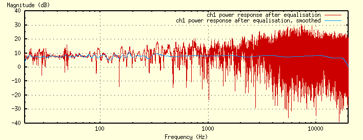
What we will measure now is the equalised power response. Ideally
it would be perfectly flat, but of course this is not the case due to
measuring errors, limited filter precision and variations in the
environment. However the result is not that bad as seen in figure 10
below. The left channel is shown there, the result is similar for the right.
|
|
Figure 10. The power response of channel 1 as measured in the
listening position after equalisation.
|
If one is not satisified with the result, one can try remaking the
filter coefficients. Increasing the number of taps is often a good
idea, but one is probably already at the machine limit. Changing the
warp factor can have some effect. Perhaps one channel is better equalised
with 127/128 while the another is best equalised with 63/64. Maybe the
room is too hard to equalise with the available processing power. One
could try to improve acoustics in the room in traditional ways
using drapes, diffusor panels etc.. There is generally no idea to try
to get the power response within less than +/- 2 dB. And of course
there is not much value in exceeding the precision of the microphone
used in the measurements. Scientifical tests have shown that a
response within +/- 1 dB is perceived as entirely flat. Being within
+/- 2 dB is still very good.
|
 |
Enjoy!
At last! Now we are finished with our task. We have equalised our
HiFi-system with good precision, yeilding a near-flat power response
in the listening position. How much better/worse does it sound then? Well we
can test for ourselves by toggling equalisation when we
listen to music. To do so you send the hangup signal to the process (kill -HUP
<pid>). If you use the large buffer, the change will lag
some time. The amplification is kept so there is no difference in
volume when the filter is turned off. Nwfiir is a multi-process
application, so the hangup signal should be sent to the parent process, that
is the process with the lowest pid.
Okay, okay, so the sound does not sound better than before, but a at
least a lot different. If the WFIR filter is used to equalise more or
less the whole range as in the example here, the sound will
get too bright. However, I did not know that when I wrote the above
text, and I don't feel like rewriting it at this time. The problem is
that a simple power response measurement only
matches the what the ear hears in the bass range. Higher up in
frequency shorter windows must be used, and one can apply various
other psycho-acoustic stuff to the filter design process. I will
(hopefully) provide a proper psycho-acoustic designer later on (it
will be FIR filter based though, WFIR filters is best for fixing only
the bass response anyway).
For now, apply the correction only up to 500
- 1000 Hz. What you will get if you do like this, is a
sound that does not sound entirely different from the unfiltered,
however the problems with standing waves in the bass range will be
almost entirely gone. These problems are very easy to notice even for
the novice, some bass tones sound much louder than others. Not only
the bass will sound better with the filter applied, but also the
higher frequencies since they are not drenched in over-amplified bass sounds. Personally I have configured
the filter this way (amplitude correction up to 700 Hz), and nowdays I don't play a CD without having the
filter activated.
|
Tips &
tricks
In this section a number of asorted tips and tricks of how to use nwfiir audio
tools are presented.
|
Over-amplify for better results
As mentioned earlier, it is necessary to set the overall amplification
of the filter to minus the top value of the filter. Or else overflow
may occur. This is a problem, since when lowering amplification in the
digital domain, we get closer to the noise floor both digitally and
analogly. However, you can cheat. Many recordings does not use the
entire digital range on the recording. This is true for almost all
classical music recordings. You can probably leave the the nwfiir
amplification to 0 dB without a single overflow. If an overflow
would occur, the sample is saturated to the maximum value (and a
warning is printed to the screen). I use my filter with 0 dB
amplification, (filter top is +3 dB) and I overflow is experienced in
only a few of my recordings, and then at the most extreme fortes. If
you manage to hear that a sample is saturated at these occations, you
probably should be employed as an expert listener somewhere. I can't
hear it.
|
|
Playing MP3 files through the equaliser
Below an example of how to play an ordinary 44.1 kHz stereo MP3 through the filter:
mpg123 -s schnittke.mp3 ¦ nwfiir -b 16s2l0,16s2l0 -o 0,0 -s
2048 wfir coeffs200.dat -4 wfir coeffs200.dat -4
The application mpg123 is a common mp3 player, and the switch
-s makes it write its output on stdout, so it can be piped to
another program. nwfiir always takes input from stdin and
write the output to stdout. aplay is ALSAs sound player
that can take raw input data on stdin and then play it through the
sound board in the computer. Since I only have a 16 bit sound board of
low quality (yes it is a SoundBlaster) I have to set the filter output
to 16 bit, thus losing quality due to requantisation error.
The filter wants each channel to be specified with three parameters,
filter type, coefficient file, and gain in dB. The filter type in this
example is wfir. Our coefficient file is coeffs200.dat, and since
its largest amplification is 4 dB, to be on the safe side we must
amplify the input with -4 dB.
|
|
Equalising a wav-file
If you do not have a fast enough machine, or want to run in
non-realtime mode by any other reason, you may do so, by piping the
output to a file. Then it may be a good idea to use large buffers.
Below is a trick how get a filtered copy of a 16 bit stereo
.wav file. You script lovers out there can probably make a
smart script out of this. The trick is to copy the header which is 44
bytes, and process the rest normally.
head -c 44 input.wav > output.wav
tail -c <input.wav file size - 44> input.wav ¦ nwfiir -b 16s2l0,16s2l0 wfir coeffs200.dat -4 wfir coeffs200.dat -4 >> output.wav
|
|
Using the computer's CD-ROM
drive as signal source
Perhaps you do not have a digital output on your HiFi-system's
CD-player, or maybe you don't own any at all. Then you could use your
CD-ROM drive in your computer running the filter software
instead. For this you can use cdparanoia.
To play a CD the command line could look something like this:
cdparanoia -r 1- - ¦ nwfiir -l -b 16s2l0,16s2l0 -o 0,0 -s 2048 \
wfir coeffs200.dat -4 wfir coeffs200.dat -4
|
Download!
You can download release 0s which
contains the source code that hopefully is possible to compile and
run. I run Debian Linux with kernel 2.2.13, and this early (yeah right) release
is made on a it-works-for-me basis. You will need the
GNU Scientific Library
installed on your system to be able to compile, I used version 0.6. Also, since nwfiir uses
IA32 assembler, you must have an
Intel processor, or combatible.
It is highly recommended that you have ALSA
installed on your machine, so you can compile nwfiir with support for
it. It is currently compatible only with the latest pre-0.6 found in
the ALSA CVS.
If you get into any trouble, just
send an email to me, and I will
help you out if I can. The code is licensed under the
GNU General Public License.
If you have an idea or want to help with something, I would like to
hear from you. The code exists for you to tinker with.
Acknowledgement
Since I am not an expert on digital signal processing, I have been
depending on help from other people. The help I have got comes mainly
from Marni Tyril. Without his help, I would not have been able to
produce this software. Also, I have had great use of the references
given below.
References
- W. T. Chu, "Impulse-Response and Reverbation-Decay Measurements Made
by Using a Periodic Pseudorandom Sequence", Applied Acoustics v
29 n 3 1990 p 193-205
- A. Härmä, "Audio Coding
with warped predictive methods", Licentiate's thesis, 1998.
- A. Härmä and M. Karjalainen, WarpTB - Matlab
Toolbox for Warped DSP (pre-pre-release), A Matlab toolbox, June
1999.
- L. G. Johansen and P. Rubak, "Target Functions and Preprocessing Techniques in Digital
Equalisation Design", AES 106th Convention, May 1999.
- J. A. Pedersen, P. Rubak and M. Tyril, "Digital
Filters for Low Frequency Equalization", AES 106th Convention, May 1999.
- K. Pedersen, T. B. Sivertsen, and M. Tyril, "Digital
Equalization Techniques for Loudspeaker and Room", Master Thesis, Aalborg
University, June 1998.
- J. Vanderkooy, "Aspects of MLS Measuring Systems",
Journal of the Audio Engineering Society v 42 n 4 April 1994 p
219-231.
|
|